Tacrolimus (Wang 2019)
Source:vignettes/articles/Wang_2019b_tacrolimus.Rmd
Wang_2019b_tacrolimus.RmdModel and source
- Citation: Wang D, Chen X, Xu H, Li Z. Population pharmacokinetics of tacrolimus in pediatric patients with systemic-onset juvenile idiopathic arthritis: Initial dosage recommendations. Exp Ther Med. 2019;18(6):4653-4660. doi:10.3892/etm.2019.8129.
- Description: One-compartment population PK model with first-order absorption for oral tacrolimus whole-blood trough concentrations in Chinese pediatric patients with systemic-onset juvenile idiopathic arthritis (Wang 2019). The absorption rate constant ka is fixed at 4.48 1/h from the literature because only trough concentrations were available. Apparent oral clearance CL/F is allometrically scaled by body weight (fixed exponent 0.75, reference 70 kg) and reduced by three fractional co-medication effects (omeprazole -36.2%, loratadine -32.2%, diltiazem -30.7%). Apparent volume V/F is scaled linearly by body weight (fixed exponent 1). Exponential IIV on CL/F only; additive residual error.
- Article: https://doi.org/10.3892/etm.2019.8129 (open access, PMC6861867)
Wang et al. (2019) fitted a one-compartment model with first-order absorption to routine therapeutic-drug-monitoring trough concentrations of oral tacrolimus in children with systemic-onset juvenile idiopathic arthritis (SOJIA), and used Monte Carlo simulation to recommend weight-banded initial doses. Because only troughs were available, the absorption rate constant was fixed at 4.48 1/h from a pediatric liver-transplant model (Yang 2015, the paper’s reference 15).
Population
Seventeen Chinese pediatric SOJIA patients (8 male, 9 female) treated at the Children’s Hospital of Fudan University between 2014 and 2017 contributed 86 whole-blood trough concentrations (1.3-9.2 ng/mL, Emit 2000 assay). From Table I: age median 9.50 (range 3.20-14.60) years, weight median 33.60 (13.50-46.00) kg, daily tacrolimus dose median 1.50 (1.00-4.00) mg. Table II lists the co-medications; omeprazole (6/17), loratadine (5/17) and diltiazem (3/17) were retained as covariates on CL/F.
Source trace
| Element | Value | Source |
|---|---|---|
| Structure: 1-compartment, first-order absorption and elimination | – | Methods, PPK modeling; Results, Modeling |
lka |
4.48 1/h (fixed) | Table III; Methods (ref 15) |
lcl |
29.7 L/h | Table III; Results equation vi |
lvc |
1120 L | Table III; Results equation vii |
e_wt_cl |
0.75 (fixed), reference 70 kg | Methods equation iii |
e_wt_vc |
1 (fixed), reference 70 kg | Methods equation iii; Results equation vii |
e_conmed_omeprazole_cl |
-0.362 | Table III; equation vi |
e_conmed_loratadine_cl |
-0.322 | Table III; equation vi |
e_conmed_diltiazem_cl |
-0.307 | Table III; equation vi |
Co-medication form (1 + theta * COV)
|
– | Methods equation v; equation vi |
etalcl |
0.265^2 = 0.070225 | Table III (omega CL/F = 0.265, read as SD; see below) |
Exponential IIV P = TV * exp(eta)
|
– | Methods equation i |
addSd |
1.229 ng/mL | Table III (sigma1, additive); Methods equation ii |
Virtual cohort and simulation
Table IV simulates 1,000 virtual patients without co-medication at
each of nine body weights and four regimens and reports the median
trough concentration, its 2.5-97.5th percentiles, and the probability of
a trough within the 1.7-5 ng/mL target range. We replicate it with 200
subjects per weight-by-regimen arm (the package cap), simulating 14 days
of dosing and reading the trough at the end of the last dosing interval.
The model’s Cc output is the individual prediction (no
residual error), which is what Table IV summarises.
The “1/0.5 mg q24h” regimen is read as 1 mg and 0.5 mg given 12 h apart within each 24 h (1.5 mg/day). The trough reported is the one before the 1 mg dose (i.e., 12 h after the 0.5 mg dose); see Assumptions.
mod <- readModelDb("Wang_2019b_tacrolimus")

weights <- c(5, 15, 20, 25, 30, 35, 40, 45, 50)
nsub <- 200
ndays <- 14

regimens <- tibble::tribble(
  ~regimen,         ~amt1, ~amt2, ~tau,
  "0.5 mg q24h",    0.5,   0,     24,
  "0.5 mg q12h",    0.5,   0.5,   12,
  "1/0.5 mg q24h",  1,     0.5,   12,
  "1 mg q12h",      1,     1,     12
)

make_arm <- function(reg, wt, id0) {
  ids <- id0 + seq_len(nsub)
  if (reg$regimen == "0.5 mg q24h") {
    dtimes <- seq(0, by = 24, length.out = ndays)
    damt <- rep(reg$amt1, ndays)
  } else {
    dtimes <- seq(0, by = 12, length.out = 2 * ndays)
    damt <- rep(c(reg$amt1, reg$amt2), ndays)
  }
  tobs <- ndays * 24
  dose <- tidyr::expand_grid(id = ids, k = seq_along(dtimes)) |>
    mutate(time = dtimes[k], amt = damt[k], evid = 1L, cmt = "depot") |>
    select(-k)
  obs <- tibble(id = ids, time = tobs, amt = 0, evid = 0L, cmt = "central")
  bind_rows(dose, obs) |>
    mutate(
      WT = wt, CONMED_OMEPRAZOLE = 0, CONMED_LORATADINE = 0,
      CONMED_DILTIAZEM = 0, regimen = reg$regimen
    )
}

arms <- list()
id0 <- 0
for (i in seq_len(nrow(regimens))) {
  for (wt in weights) {
    arms[[length(arms) + 1]] <- make_arm(regimens[i, ], wt, id0)
    id0 <- id0 + nsub
  }
}
ev <- bind_rows(arms) |> arrange(id, time, desc(evid))

rxode2::rxSetSeed(2019)
sim <- rxode2::rxSolve(mod, events = ev, keep = c("WT", "regimen"))
#> ℹ parameter labels from comments will be replaced by 'label()'
trough <- as.data.frame(sim) |> filter(time == ndays * 24)
published <- tibble::tribble(
  ~WT, ~regimen,         ~pub_med, ~pub_lo, ~pub_hi, ~pub_pta,
  50,  "0.5 mg q24h",    0.61, 0.30, 1.13,  0,
  45,  "0.5 mg q24h",    0.65, 0.32, 1.23,  0,
  40,  "0.5 mg q24h",    0.71, 0.34, 1.34,  0,
  35,  "0.5 mg q24h",    0.77, 0.37, 1.48,  0.9,
  30,  "0.5 mg q24h",    0.86, 0.41, 1.66,  1.9,
  25,  "0.5 mg q24h",    0.96, 0.45, 1.90,  5.3,
  20,  "0.5 mg q24h",    1.11, 0.51, 2.23, 12.0,
  15,  "0.5 mg q24h",    1.33, 0.59, 2.74, 22.5,
  5,   "0.5 mg q24h",    2.57, 1.00, 5.82, 77.2,
  50,  "0.5 mg q12h",    1.51, 0.80, 2.58, 35.3,
  45,  "0.5 mg q12h",    1.63, 0.85, 2.81, 45.4,
  40,  "0.5 mg q12h",    1.78, 0.93, 3.08, 55.9,
  35,  "0.5 mg q12h",    1.96, 1.01, 3.41, 67.7,
  30,  "0.5 mg q12h",    2.19, 1.12, 3.85, 79.4,
  25,  "0.5 mg q12h",    2.49, 1.27, 4.42, 88.0,
  20,  "0.5 mg q12h",    2.92, 1.47, 5.24, 89.7,
  15,  "0.5 mg q12h",    3.57, 1.77, 6.52, 82.7,
  5,   "0.5 mg q12h",    7.59, 3.54, 14.64, 12.2,
  50,  "1/0.5 mg q24h",  2.14, 1.08, 3.75, 77.1,
  45,  "1/0.5 mg q24h",  2.31, 1.16, 4.07, 83.3,
  40,  "1/0.5 mg q24h",  2.51, 1.25, 4.45, 87.5,
  35,  "1/0.5 mg q24h",  2.75, 1.36, 4.93, 89.1,
  30,  "1/0.5 mg q24h",  3.07, 1.50, 5.55, 87.9,
  25,  "1/0.5 mg q24h",  3.48, 1.69, 6.37, 83.1,
  20,  "1/0.5 mg q24h",  4.06, 1.94, 7.54, 71.6,
  15,  "1/0.5 mg q24h",  4.94, 2.32, 9.33, 50.9,
  5,   "1/0.5 mg q24h", 10.25, 4.45, 20.66, 4.9,
  50,  "1 mg q12h",      3.03, 1.59, 5.17, 92.1,
  45,  "1 mg q12h",      3.27, 1.71, 5.61, 89.8,
  40,  "1 mg q12h",      3.56, 1.85, 6.15, 89.5,
  35,  "1 mg q12h",      3.92, 2.03, 6.83, 77.3,
  30,  "1 mg q12h",      4.37, 2.25, 7.69, 65.3,
  25,  "1 mg q12h",      4.98, 2.53, 8.85, 50.5,
  20,  "1 mg q12h",      5.83, 2.94, 10.49, 31.7,
  15,  "1 mg q12h",      7.13, 3.54, 13.03, 13.7,
  5,   "1 mg q12h",     15.18, 7.08, 29.27, 0.1
)

simsum <- trough |>
  group_by(WT, regimen) |>
  summarise(
    sim_med = median(Cc),
    sim_lo = quantile(Cc, 0.025),
    sim_hi = quantile(Cc, 0.975),
    sim_pta = 100 * mean(Cc >= 1.7 & Cc <= 5),
    .groups = "drop"
  )

cmp4 <- inner_join(published, simsum, by = c("WT", "regimen")) |>
  mutate(pct_diff_med = 100 * (sim_med - pub_med) / pub_med)

cmp4 |>
  mutate(
    Published = sprintf("%.2f (%.2f-%.2f); %.1f%%", pub_med, pub_lo, pub_hi, pub_pta),
    Simulated = sprintf("%.2f (%.2f-%.2f); %.1f%%", sim_med, sim_lo, sim_hi, sim_pta)
  ) |>
  select(regimen, WT, Published, Simulated, pct_diff_med) |>
  arrange(regimen, WT) |>
  dplyr::rename(
    "Regimen" = regimen, "Weight (kg)" = WT,
    "Published median (95% range); P(1.7-5 ng/mL)" = Published,
    "Simulated median (95% range); P(1.7-5 ng/mL)" = Simulated,
    "Median % diff" = pct_diff_med
  ) |>
knitr::kable(digits = 1, caption = "Replicates Table IV of Wang 2019 (trough concentrations in ng/mL, no co-medication).")| Regimen | Weight (kg) | Published median (95% range); P(1.7-5 ng/mL) | Simulated median (95% range); P(1.7-5 ng/mL) | Median % diff |
|---|---|---|---|---|
| 0.5 mg q12h | 5 | 7.59 (3.54-14.64); 12.2% | 7.24 (3.28-14.00); 14.5% | -4.6 |
| 0.5 mg q12h | 15 | 3.57 (1.77-6.52); 82.7% | 3.56 (1.77-6.69); 82.5% | -0.4 |
| 0.5 mg q12h | 20 | 2.92 (1.47-5.24); 89.7% | 2.82 (1.49-5.22); 88.5% | -3.3 |
| 0.5 mg q12h | 25 | 2.49 (1.27-4.42); 88.0% | 2.45 (1.20-4.28); 85.5% | -1.7 |
| 0.5 mg q12h | 30 | 2.19 (1.12-3.85); 79.4% | 2.21 (1.12-3.90); 80.0% | 1.1 |
| 0.5 mg q12h | 35 | 1.96 (1.01-3.41); 67.7% | 1.96 (1.02-3.42); 67.5% | 0.0 |
| 0.5 mg q12h | 40 | 1.78 (0.93-3.08); 55.9% | 1.78 (1.04-3.34); 56.0% | -0.2 |
| 0.5 mg q12h | 45 | 1.63 (0.85-2.81); 45.4% | 1.62 (0.96-2.79); 43.0% | -0.9 |
| 0.5 mg q12h | 50 | 1.51 (0.80-2.58); 35.3% | 1.51 (0.86-2.71); 37.5% | 0.2 |
| 0.5 mg q24h | 5 | 2.57 (1.00-5.82); 77.2% | 2.67 (0.90-5.98); 77.5% | 4.1 |
| 0.5 mg q24h | 15 | 1.33 (0.59-2.74); 22.5% | 1.32 (0.58-2.87); 28.0% | -1.0 |
| 0.5 mg q24h | 20 | 1.11 (0.51-2.23); 12.0% | 1.10 (0.48-2.33); 14.0% | -1.3 |
| 0.5 mg q24h | 25 | 0.96 (0.45-1.90); 5.3% | 0.96 (0.41-1.87); 6.5% | -0.2 |
| 0.5 mg q24h | 30 | 0.86 (0.41-1.66); 1.9% | 0.88 (0.36-1.70); 3.0% | 2.1 |
| 0.5 mg q24h | 35 | 0.77 (0.37-1.48); 0.9% | 0.78 (0.40-1.59); 1.0% | 1.4 |
| 0.5 mg q24h | 40 | 0.71 (0.34-1.34); 0.0% | 0.72 (0.34-1.40); 0.5% | 1.4 |
| 0.5 mg q24h | 45 | 0.65 (0.32-1.23); 0.0% | 0.68 (0.27-1.35); 0.0% | 4.3 |
| 0.5 mg q24h | 50 | 0.61 (0.30-1.13); 0.0% | 0.61 (0.31-1.20); 0.0% | 0.7 |
| 1 mg q12h | 5 | 15.18 (7.08-29.27); 0.1% | 15.25 (7.21-27.13); 0.0% | 0.5 |
| 1 mg q12h | 15 | 7.13 (3.54-13.03); 13.7% | 7.08 (3.29-13.10); 16.0% | -0.7 |
| 1 mg q12h | 20 | 5.83 (2.94-10.49); 31.7% | 5.61 (3.18-10.42); 33.5% | -3.7 |
| 1 mg q12h | 25 | 4.98 (2.53-8.85); 50.5% | 5.06 (2.62-8.78); 47.0% | 1.6 |
| 1 mg q12h | 30 | 4.37 (2.25-7.69); 65.3% | 4.27 (2.52-7.69); 73.0% | -2.2 |
| 1 mg q12h | 35 | 3.92 (2.03-6.83); 77.3% | 3.89 (1.97-6.61); 78.5% | -0.7 |
| 1 mg q12h | 40 | 3.56 (1.85-6.15); 89.5% | 3.62 (1.72-5.97); 86.0% | 1.6 |
| 1 mg q12h | 45 | 3.27 (1.71-5.61); 89.8% | 3.41 (1.79-6.06); 91.0% | 4.2 |
| 1 mg q12h | 50 | 3.03 (1.59-5.17); 92.1% | 3.12 (1.75-5.30); 94.5% | 2.9 |
| 1/0.5 mg q24h | 5 | 10.25 (4.45-20.66); 4.9% | 10.20 (3.95-19.71); 5.0% | -0.5 |
| 1/0.5 mg q24h | 15 | 4.94 (2.32-9.33); 50.9% | 5.11 (2.61-9.71); 45.5% | 3.4 |
| 1/0.5 mg q24h | 20 | 4.06 (1.94-7.54); 71.6% | 4.22 (1.80-7.83); 64.0% | 4.0 |
| 1/0.5 mg q24h | 25 | 3.48 (1.69-6.37); 83.1% | 3.67 (1.72-6.23); 86.0% | 5.4 |
| 1/0.5 mg q24h | 30 | 3.07 (1.50-5.55); 87.9% | 2.99 (1.51-6.08); 88.0% | -2.4 |
| 1/0.5 mg q24h | 35 | 2.75 (1.36-4.93); 89.1% | 2.85 (1.30-4.87); 90.5% | 3.7 |
| 1/0.5 mg q24h | 40 | 2.51 (1.25-4.45); 87.5% | 2.55 (1.11-4.80); 88.5% | 1.5 |
| 1/0.5 mg q24h | 45 | 2.31 (1.16-4.07); 83.3% | 2.41 (0.99-4.90); 83.5% | 4.4 |
| 1/0.5 mg q24h | 50 | 2.14 (1.08-3.75); 77.1% | 2.18 (1.01-4.21); 72.5% | 1.7 |
# Medians are driven by the typical values (CL/F, V/F, allometry) and the
# regimen reading; a mis-transcribed parameter would move them by tens of
# percent. The envelope check uses the 90th percentile of |% diff| rather than
# the maximum (robust to Monte Carlo noise at n = 200).
stopifnot(
  abs(median(cmp4$pct_diff_med)) < 5,
  quantile(abs(cmp4$pct_diff_med), 0.9) < 10
)
ggplot(cmp4, aes(WT)) +
  geom_ribbon(aes(ymin = sim_lo, ymax = sim_hi), fill = "steelblue", alpha = 0.25) +
  geom_line(aes(y = sim_med), colour = "steelblue") +
  geom_pointrange(aes(y = pub_med, ymin = pub_lo, ymax = pub_hi), size = 0.2) +
  geom_hline(yintercept = c(1.7, 5), linetype = "dashed") +
  facet_wrap(~regimen, scales = "free_y") +
  labs(x = "Body weight (kg)", y = "Trough tacrolimus (ng/mL)")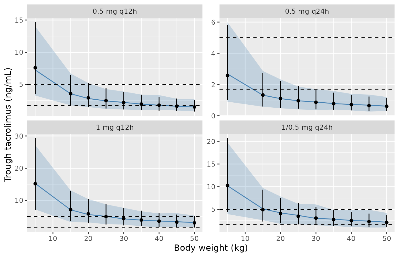
Simulated trough concentration by body weight and regimen (median and 2.5-97.5th percentiles, lines/ribbons) against Wang 2019 Table IV (points and error bars). Dashed lines: 1.7-5 ng/mL target range. Replicates Table IV of Wang 2019.
Co-medication effects
Typical CL/F at 30 kg with each retained co-medication (equation vi).
comed <- tibble::tribble(
  ~scenario,         ~CONMED_OMEPRAZOLE, ~CONMED_LORATADINE, ~CONMED_DILTIAZEM,
  "none",            0, 0, 0,
  "omeprazole",      1, 0, 0,
  "loratadine",      0, 1, 0,
  "diltiazem",       0, 0, 1
) |>
  mutate(cl_typ = 29.7 * (30 / 70)^0.75 * (1 - 0.362 * CONMED_OMEPRAZOLE) *
    (1 - 0.322 * CONMED_LORATADINE) * (1 - 0.307 * CONMED_DILTIAZEM))
knitr::kable(comed |> dplyr::rename("Scenario" = scenario, "Typical CL/F (L/h)" = cl_typ), digits = 2)| Scenario | CONMED_OMEPRAZOLE | CONMED_LORATADINE | CONMED_DILTIAZEM | Typical CL/F (L/h) |
|---|---|---|---|---|
| none | 0 | 0 | 0 | 15.73 |
| omeprazole | 1 | 0 | 0 | 10.04 |
| loratadine | 0 | 1 | 0 | 10.67 |
| diltiazem | 0 | 0 | 1 | 10.90 |
PKNCA validation
The paper reports no NCA. As a structural check, typical-value
subjects (zeroRe()) at each Table IV weight receive 0.5 mg
q12h for 14 days; PKNCA computes the steady-state AUC over the last
dosing interval, which must equal the closed form
Dose / (CL/F), and the steady-state Cmin is compared with
the Table IV median trough.
mod_typ <- rxode2::zeroRe(mod)
#> ℹ parameter labels from comments will be replaced by 'label()'
tlast <- (2 * ndays - 1) * 12
ev_nca <- lapply(seq_along(weights), function(i) {
  dose <- tibble(
    id = i, time = seq(0, by = 12, length.out = 2 * ndays), amt = 0.5,
    evid = 1L, cmt = "depot"
  )
  obs <- tibble(
    id = i, time = sort(unique(c(tlast + c(0, 0.25, 0.5, 1, 1.5, 2, 3, 4, 6, 8, 10, 12)))),
    amt = 0, evid = 0L, cmt = "central"
  )
  bind_rows(dose, obs) |> mutate(WT = weights[i])
}) |>
  bind_rows() |>
  mutate(CONMED_OMEPRAZOLE = 0, CONMED_LORATADINE = 0, CONMED_DILTIAZEM = 0) |>
  arrange(id, time, desc(evid))

sim_nca <- rxode2::rxSolve(mod_typ, events = ev_nca, keep = "WT") |>
  as.data.frame() |>
  mutate(treatment = paste0(WT, " kg"))
#> ℹ omega/sigma items treated as zero: 'etalcl'
#> Warning: multi-subject simulation without without 'omega'

conc <- sim_nca |>
  filter(!is.na(Cc), time >= tlast) |>
  select(id, time, Cc, treatment)
doses <- ev_nca |>
  filter(evid == 1, time == tlast) |>
  mutate(treatment = paste0(WT, " kg")) |>
  select(id, time, amt, treatment)

o_conc <- PKNCAconc(conc, Cc ~ time | treatment + id)
o_dose <- PKNCAdose(doses, amt ~ time | treatment + id)
intervals <- data.frame(start = tlast, end = tlast + 12, auclast = TRUE, cmin = TRUE, cmax = TRUE)
nca_res <- pk.nca(PKNCAdata(o_conc, o_dose, intervals = intervals))

nca_wide <- as.data.frame(nca_res) |>
  select(treatment, PPTESTCD, PPORRES) |>
  tidyr::pivot_wider(names_from = PPTESTCD, values_from = PPORRES) |>
  mutate(
    WT = as.numeric(sub(" kg", "", treatment)),
    auc_closed = 1000 * 0.5 / (29.7 * (WT / 70)^0.75)
  ) |>
  left_join(filter(published, regimen == "0.5 mg q12h") |> select(WT, pub_med), by = "WT") |>
  arrange(WT)

nca_wide |>
  select(WT, auclast, auc_closed, cmax, cmin, pub_med) |>
  dplyr::rename(
    "Weight (kg)" = WT, "AUCtau (PKNCA, ng*h/mL)" = auclast,
    "Dose/(CL/F) (ng*h/mL)" = auc_closed, "Cmax (ng/mL)" = cmax,
    "Cmin (ng/mL)" = cmin, "Table IV median trough (ng/mL)" = pub_med
  ) |>
knitr::kable(digits = 2, caption = "Typical-value steady-state NCA, 0.5 mg q12h.")| Weight (kg) | AUCtau (PKNCA, ng*h/mL) | Dose/(CL/F) (ng*h/mL) | Cmax (ng/mL) | Cmin (ng/mL) | Table IV median trough (ng/mL) |
|---|---|---|---|---|---|
| 5 | 121.66 | 121.85 | 13.00 | 7.43 | 7.59 |
| 15 | 53.39 | 53.45 | 5.39 | 3.52 | 3.57 |
| 20 | 43.03 | 43.08 | 4.29 | 2.89 | 2.92 |
| 25 | 36.40 | 36.44 | 3.59 | 2.47 | 2.49 |
| 30 | 31.75 | 31.78 | 3.11 | 2.18 | 2.19 |
| 35 | 28.29 | 28.31 | 2.76 | 1.95 | 1.96 |
| 40 | 25.59 | 25.61 | 2.48 | 1.78 | 1.78 |
| 45 | 23.43 | 23.45 | 2.26 | 1.64 | 1.63 |
| 50 | 21.65 | 21.67 | 2.08 | 1.52 | 1.51 |
Assumptions and deviations
- IIV scale. Table III reports “omega CL/F = 0.265” without stating whether it is a variance or an SD. Simulating Table IV under both readings settles it: with omega = 0.265 as the SD of eta (variance 0.070225) the simulated 2.5-97.5th percentiles reproduce Table IV (e.g. 30 kg, 0.5 mg q12h: 1.12-3.97 vs published 1.12-3.85), whereas treating 0.265 as the variance widens them roughly three-fold (0.54-6.82). The SD reading is used.
- Residual error scale. sigma1 = 1.229 (additive) is taken as an SD in ng/mL, consistent with the SD convention established for omega above. The paper offers no independent check; if it were a variance the SD would be 1.109 ng/mL. It does not affect the Table IV replication, which excludes residual error (the published lower percentiles, e.g. 0.30 ng/mL, would be negative with an additive SD of about 1.2 ng/mL included).
- “1/0.5 mg q24h” regimen. Interpreted as 1 mg and 0.5 mg 12 h apart each day with the trough taken before the 1 mg dose. The paper does not define the notation; the resulting medians match Table IV.
- Target attainment. The Table IV probability is read as P(1.7 ng/mL <= trough <= 5 ng/mL).
- Co-medication indicators. The paper does not state whether the omeprazole / loratadine / diltiazem indicators were time-varying; they are accepted per record.
- Fixed ka is inherited from Yang 2015 (pediatric liver transplantation) and is not identifiable from trough-only data.
- The body-weight reference (70 kg) lies outside the observed range (13.5-46 kg); the typical CL/F of 29.7 L/h is therefore an extrapolated adult-equivalent value, as the authors state.