Iclaprim (Lodise 2018) • nlmixr2lib

Model and source

Citation: Lodise TP, Bosso J, Kelly C, Williams PJ, Lane JR, Huang DB. Pharmacokinetic and pharmacodynamic analyses to determine the optimal fixed dosing regimen of iclaprim for treatment of patients with serious infections caused by Gram-positive pathogens. Antimicrob Agents Chemother. 2018;62(4):e01184-17. doi:10.1128/AAC.01184-17.
Description: Two-compartment IV-infusion population PK model for iclaprim, a bacterial dihydrofolate reductase inhibitor, in adult patients with complicated skin and skin-structure infections from the pooled ASSIST-1 and ASSIST-2 phase 3 trials (Lodise 2018). Structural typical-value equations are additive-linear (NONMEM theta-sum form rather than power form): central volume V1 carries a body-weight slope; clearance CL carries age + sex (male shift) + sampling-occasion (day 1-2 vs day 4 +/- 1) shifts; peripheral volume V2 has no covariates; inter-compartmental clearance Q carries a severe-cSSSI-infection shift. Block-correlated log-normal IIV on V1, CL, V2 was retained in the source paper but only diagonal CV% values are tabulated – off-diagonal covariances are not reported and are implemented here as diagonal-only (documented in the vignette Assumptions and deviations section). Combined proportional + additive residual error.
Article: https://doi.org/10.1128/AAC.01184-17

Population

Lodise et al. 2018 developed a population PK model of iclaprim, a bacterial dihydrofolate reductase inhibitor, from pooled data of the ASSIST-1 and ASSIST-2 phase 3 trials in adults with complicated skin and skin-structure infections (cSSSI). 470 patients (241 from ASSIST-1 and 235 from ASSIST-2) contributed 3,061 plasma iclaprim concentrations to the model fit; subjects were sampled on two occasions per protocol – the first occasion after the first dose (day 1) and the second occasion on day 4 (+/- 1 day) of treatment. Across both trials, iclaprim was administered at 0.8 mg/kg infused intravenously over 0.5 h every 12 h for 8 to 14 days.

Baseline demographics (Lodise 2018 Table 3): weight 42-143 kg (mean 79 +/- 17.1, median 76 kg), height 1.29-1.96 m, BMI 16.8-54.7 kg/m^2, ideal weight 28.8-89.5 kg, age 18-87 years (mean 47.8 +/- 15.3, median 47.5 years), Cockcroft-Gault creatinine clearance 18-172 mL/min (mean 99 +/- 29), ALT 0.04-245 SI units (mean 13.4 +/- 21.6), total bilirubin 1.7-40.9 SI units (mean 7.5 +/- 5.4). Patients with BMI > 40 and patients with estimated creatinine clearance < 30 mL/min were excluded from the ASSIST studies. Disease-severity classification (severe vs not severe cSSSI) was retained as a covariate on inter-compartmental clearance Q in the final model.

The same metadata is available programmatically via readModelDb("Lodise_2018_iclaprim")()$population.

Source trace

The per-parameter origin is recorded inline next to each ini() entry in inst/modeldb/specificDrugs/Lodise_2018_iclaprim.R. The table below collects them in one place for review.

Equation / parameter	Value	Source location
`lcl` (CL intercept at AGE=0, female, day 1-2, non-severe, L/h)	`log(36.1)`	Lodise 2018 Table 1: theta2 = 36.1 (SE 2.04; 95% CI 32.02-40.18)
`lvc` (V1 intercept at WT=0, L)	`log(48.2)`	Lodise 2018 Table 1: theta1 = 48.2 (SE 4.22; 95% CI 39.76-56.64)
`lvp` (V2, L)	`log(36.8)`	Lodise 2018 Table 1: theta3 = 36.8 (SE 2.62; 95% CI 31.56-42.04)
`lq` (Q intercept at non-severe, L/h)	`log(1.85)`	Lodise 2018 Table 1: theta4 = 1.85 (SE 0.851; 95% CI 0.148-3.552)
`e_age_cl` (additive slope on CL, L/h per year)	`-0.210`	Lodise 2018 Table 1: theta5 = -0.210 (SE 0.031; 95% CI -0.272 to -0.148)
`e_wt_vc` (additive slope on V1, L per kg)	`0.353`	Lodise 2018 Table 1: theta6 = 0.353 (SE 0.046; 95% CI 0.261-0.445)
`e_sex_cl` (additive male shift on CL, L/h; applied as `(1 - SEXF)`)	`2.78`	Lodise 2018 Table 1: theta7 = 2.78 (SE 1.06; 95% CI 0.66-4.90)
`e_occ_cl` (additive day-4 shift on CL, L/h)	`3.97`	Lodise 2018 Table 1: theta9 = 3.97 (SE 0.694; 95% CI 2.58-5.36)
`e_infect_csssi_sev_q` (additive severe-cSSSI shift on Q, L/h)	`13.5`	Lodise 2018 Table 1: theta8 = 13.5 (SE 2.29; 95% CI 8.92-18.08)
`etalcl` (omega_CL, log-normal variance)	`0.15543` (41% CV)	Lodise 2018 Table 1: CV% 41 on CL (95% CI 38-44); omega^2 = log(1 + CV^2)
`etalvc` (omega_V1, log-normal variance)	`0.23107` (51% CV)	Lodise 2018 Table 1: CV% 51 on V1 (95% CI 45-56); omega^2 = log(1 + CV^2)
`etalvp` (omega_V2, log-normal variance)	`0.55362` (86% CV)	Lodise 2018 Table 1: CV% 86 on V2 (95% CI 65-104); omega^2 = log(1 + CV^2)
`propSd` (proportional residual error, fraction)	`0.365`	Lodise 2018 Table 1: residual error CV% = 36.5
`addSd` (additive residual error, ng/mL)	`5.19`	Lodise 2018 Table 1: additive residual error = 5.19 ng/mL (SE 0.87)
CL typical-value equation (`CL = theta2 + theta5 * AGE + theta7 * SEX + theta9 * OCC`)	n/a	Lodise 2018 Results, Population PK model paragraph
V1 typical-value equation (`V1 = theta1 + theta6 * WT`)	n/a	Lodise 2018 Results, Population PK model paragraph
V2 typical-value equation (`V2 = theta3`)	n/a	Lodise 2018 Results, Population PK model paragraph
Q typical-value equation (`Q = theta4 + theta8 * SOI`)	n/a	Lodise 2018 Results, Population PK model paragraph
Two-compartment ODE system	n/a	Lodise 2018 Results, “two-compartment model” + Discussion

Virtual cohort

Original observed concentrations are not publicly available. The simulations below use a virtual cohort whose covariate distributions mirror the Lodise 2018 Table 3 baseline demographics: 200 subjects in each of four dosing-regimen strata (the four regimens summarised in Lodise 2018 Table 2). All cohorts share the same underlying demographic distribution; doses differ across strata.

set.seed(2018)

N_PER_REGIMEN <- 100L
N_DOSES       <- 6L      # six q12h doses -> steady state by day 4
DOSE_INTERVAL <- 12      # hours

# Four regimens summarized in Lodise 2018 Table 2.
regimens <- list(
  list(label = "0.8 mg/kg over 0.5 h", mode = "mgkg", mg_per_kg = 0.8, dose_mg = NA_real_, t_inf_h = 0.5),
  list(label = "64 mg over 2 h",       mode = "fixed", mg_per_kg = NA_real_, dose_mg = 64, t_inf_h = 2.0),
  list(label = "72 mg over 2 h",       mode = "fixed", mg_per_kg = NA_real_, dose_mg = 72, t_inf_h = 2.0),
  list(label = "80 mg over 2 h",       mode = "fixed", mg_per_kg = NA_real_, dose_mg = 80, t_inf_h = 2.0)
)

# Sample baseline demographics for one subject, matching Lodise 2018 Table 3
# distributions (means / SDs with truncation to the reported ranges).
sample_subject <- function() {
  wt  <- pmin(pmax(rnorm(1, 79.0, 17.1), 42), 143)
  age <- pmin(pmax(rnorm(1, 47.8, 15.3), 18), 87)
  # Lodise 2018 Table 3 does not tabulate sex frequencies; the ASSIST trials
  # enrolled a mixed-sex adult cohort. Default to a 50/50 split so both branches
  # of the male-additive CL shift are exercised in the cohort.
  sexf <- rbinom(1, 1, 0.5)
  # Severe-cSSSI prevalence is not reported in Lodise 2018; the SOI binary
  # covariate is retained on Q with reference category 0 (not severe). Default
  # to a 50/50 split to exercise both Q values.
  dis  <- rbinom(1, 1, 0.5)
  data.frame(WT = wt, AGE = age, SEXF = sexf, DIS_INFECT_CSSSI_SEV = dis)
}

# Build one virtual subject's event table. The OCC covariate switches inside
# model() as a function of time: OCC = 1 for samples in the first ~48 hours and
# OCC = 2 from the start of the day-4 (+/- 1 day) window onward. The boundary
# is encoded at 3*24 = 72 h (start of "day 4") so simulation samples in days
# 1-3 carry OCC = 1 and samples from day 4 onward carry OCC = 2.
make_subject <- function(id, covs, regimen, id_offset = 0L) {
  if (regimen$mode == "mgkg") {
    dose_mg <- regimen$mg_per_kg * covs$WT
  } else {
    dose_mg <- regimen$dose_mg
  }
  rate_mg_per_h <- dose_mg / regimen$t_inf_h

  ev <- rxode2::et(
    amt  = dose_mg,
    rate = rate_mg_per_h,
    cmt  = "central",
    ii   = DOSE_INTERVAL,
    addl = N_DOSES - 1L,
    time = 0
  )
  # Sparse sampling through early doses; dense sampling across the final
  # steady-state interval (60-72 h) which is where the VPC and NCA both
  # operate. Unique() avoids a t = 60 boundary duplicate that would otherwise
  # produce duplicate (id, tad) rows in the PKNCA concentration table.
  obs_times <- sort(unique(c(
    seq(0, 60, by = 2),
    seq(60, 72, by = 0.25)
  )))
  ev <- rxode2::et(ev, obs_times)
  df <- as.data.frame(ev)

  df$WT                   <- covs$WT
  df$AGE                  <- covs$AGE
  df$SEXF                 <- covs$SEXF
  df$DIS_INFECT_CSSSI_SEV <- covs$DIS_INFECT_CSSSI_SEV
  df$OCC                  <- ifelse(df$time < 3 * 24, 1L, 2L)
  df$id                   <- id_offset + id
  df$regimen              <- regimen$label
  df$dose_mg              <- dose_mg
  df
}

events <- bind_rows(lapply(seq_along(regimens), function(ri) {
  reg <- regimens[[ri]]
  bind_rows(lapply(seq_len(N_PER_REGIMEN), function(j) {
    make_subject(
      id        = j,
      covs      = sample_subject(),
      regimen   = reg,
      id_offset = (ri - 1L) * N_PER_REGIMEN
    )
  }))
}))

stopifnot(!anyDuplicated(unique(events[, c("id", "time", "evid")])))

Simulation

mod <- readModelDb("Lodise_2018_iclaprim")()

sim <- rxode2::rxSolve(
  mod,
  events = events,
  keep   = c("regimen", "WT", "AGE", "SEXF", "DIS_INFECT_CSSSI_SEV", "OCC", "dose_mg")
) |> as.data.frame()

mod_typical <- rxode2::zeroRe(mod)
typical_events <- events |>
  group_by(regimen) |>
  filter(id == min(id)) |>
  ungroup() |>
  mutate(
    WT = 76, AGE = 47.5, SEXF = 1L,
    DIS_INFECT_CSSSI_SEV = 0L
  )
sim_typ <- rxode2::rxSolve(
  mod_typical,
  events = typical_events,
  keep   = c("regimen", "dose_mg")
) |> as.data.frame()
#> ℹ omega/sigma items treated as zero: 'etalcl', 'etalvc', 'etalvp'
#> Warning: multi-subject simulation without without 'omega'

Replicate published figures

Steady-state concentration-time profile by regimen

Lodise 2018 does not publish explicit numerical concentration-time profiles for the four dosing regimens; Table 2 summarises the regimens via their steady-state PK / PD endpoints (Cmaxss, AUC0-24ss, AUC/MIC, T > MIC). The plot below shows the simulated VPC over the steady-state dosing interval (the 12-hour window between the 5th and 6th doses, i.e. between 60 and 72 h after the first dose) for each regimen.

last_dose_t <- (N_DOSES - 1L) * DOSE_INTERVAL
sim_ss <- sim |>
  filter(time >= last_dose_t,
         time <= last_dose_t + DOSE_INTERVAL,
         !is.na(Cc), Cc > 0) |>
  mutate(tad = time - last_dose_t)

vpc_summary <- sim_ss |>
  group_by(regimen, tad) |>
  summarise(
    Q05 = quantile(Cc, 0.05, na.rm = TRUE),
    Q50 = quantile(Cc, 0.50, na.rm = TRUE),
    Q95 = quantile(Cc, 0.95, na.rm = TRUE),
    .groups = "drop"
  )

ggplot(vpc_summary, aes(tad, Q50, colour = regimen, fill = regimen)) +
  geom_ribbon(aes(ymin = Q05, ymax = Q95), alpha = 0.18, colour = NA) +
  geom_line(linewidth = 0.8) +
  labs(
    x       = "Time after start of dose-6 infusion (h)",
    y       = "Iclaprim plasma concentration (ng/mL)",
    colour  = "Regimen",
    fill    = "Regimen",
    title   = "Steady-state VPC across the four regimens of Lodise 2018 Table 2",
    caption = paste(
      "Simulated steady-state interval (5th-95th percentile ribbon, median line);",
      "compare medians at end-of-infusion to Lodise 2018 Table 2 Cmaxss column."
    )
  ) +
  theme_minimal()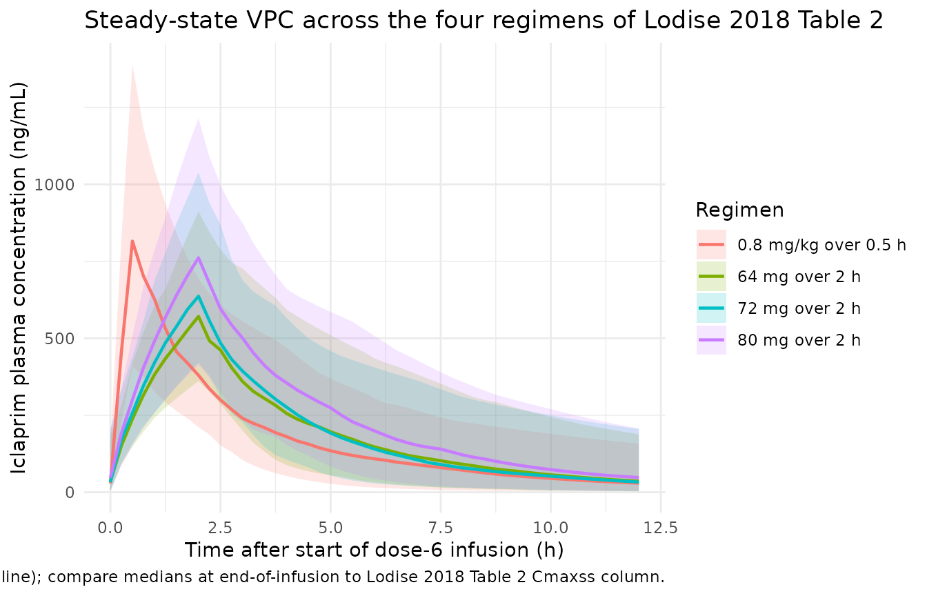

Typical-patient profile

sim_typ |>
  filter(time >= last_dose_t, time <= last_dose_t + DOSE_INTERVAL,
         !is.na(Cc), Cc > 0) |>
  mutate(tad = time - last_dose_t) |>
  ggplot(aes(tad, Cc, colour = regimen)) +
  geom_line(linewidth = 0.9) +
  labs(
    x       = "Time after start of dose-6 infusion (h)",
    y       = "Iclaprim plasma concentration (ng/mL)",
    colour  = "Regimen",
    title   = "Typical-patient iclaprim PK at steady state",
    caption = paste(
      "Typical patient: WT = 76 kg, AGE = 47.5 yr, female (SEXF = 1),",
      "not severe (DIS_INFECT_CSSSI_SEV = 0). OCC = 2 at steady state."
    )
  ) +
  theme_minimal()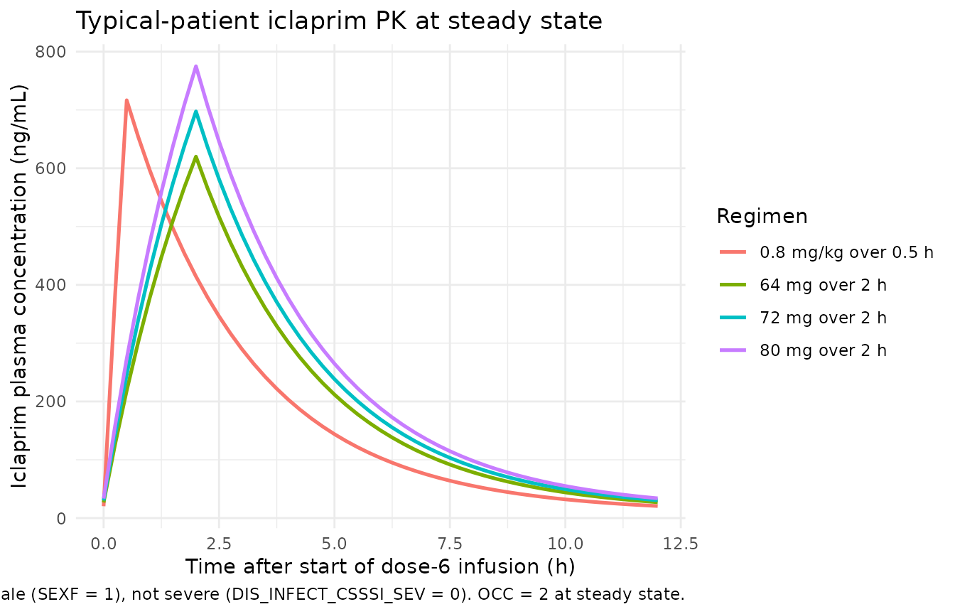

PKNCA validation

Steady-state NCA over the 12-hour dosing interval between doses 5 and 6 (the final inter-dose interval simulated). For each regimen we compute Cmaxss (maximum concentration during the steady-state interval) and AUC over the 12-hour interval; the AUC over 24 hours at steady state (AUC0-24ss in Lodise 2018 Table 2) is twice the 12-hour AUC because the regimen is q12h.

sim_nca <- sim |>
  filter(time >= last_dose_t,
         time <= last_dose_t + DOSE_INTERVAL,
         !is.na(Cc), Cc > 0) |>
  mutate(tad = time - last_dose_t) |>
  select(id, tad, Cc, regimen)

# The events table holds a single addl-encoded dose row per subject at t = 0;
# the 6th dose at t = 60 h is generated inside rxSolve via ii / addl. For the
# PKNCA dose table we represent the steady-state dose explicitly at tad = 0
# (one row per (regimen, id)) using the per-subject `amt` recorded in events.
dose_df <- events |>
  filter(evid == 1L) |>
  group_by(regimen, id) |>
  summarise(amt = first(amt), .groups = "drop") |>
  mutate(tad = 0)

conc_obj <- PKNCA::PKNCAconc(sim_nca, Cc ~ tad | regimen + id)
dose_obj <- PKNCA::PKNCAdose(dose_df, amt ~ tad | regimen + id,
                             route = "intravascular")

intervals <- data.frame(
  start    = 0,
  end      = DOSE_INTERVAL,
  cmax     = TRUE,
  tmax     = TRUE,
  auclast  = TRUE
)

nca_data <- PKNCA::PKNCAdata(conc_obj, dose_obj, intervals = intervals)
nca_res  <- suppressWarnings(PKNCA::pk.nca(nca_data))
nca_df   <- as.data.frame(nca_res$result)

nca_summary <- nca_df |>
  group_by(regimen, PPTESTCD) |>
  summarise(
    median = round(median(PPORRES, na.rm = TRUE), 1),
    p25    = round(quantile(PPORRES, 0.25, na.rm = TRUE), 1),
    p75    = round(quantile(PPORRES, 0.75, na.rm = TRUE), 1),
    .groups = "drop"
  ) |>
  pivot_wider(names_from = PPTESTCD,
              values_from = c(median, p25, p75))

knitr::kable(
  nca_summary,
  caption = "Simulated steady-state NCA parameters (median and IQR) by regimen. Cmaxss in ng/mL, auclast in ng*h/mL over the 12-h interval; AUC0-24ss = 2 * auclast."
)

Simulated steady-state NCA parameters (median and IQR) by regimen. Cmaxss in ng/mL, auclast in ngh/mL over the 12-h interval; AUC0-24ss = 2 auclast.
regimen	median_auclast	median_cmax	median_tmax	p25_auclast	p25_cmax	p25_tmax	p75_auclast	p75_cmax	p75_tmax
0.8 mg/kg over 0.5 h	2250.7	815.5	0.5	1653.7	614.0	0.5	3026.3	964.8	0.5
64 mg over 2 h	2345.4	571.1	2.0	1830.7	461.7	2.0	3189.0	731.9	2.0
72 mg over 2 h	2533.1	636.6	2.0	1882.7	509.1	2.0	3510.5	822.6	2.0
80 mg over 2 h	3218.4	761.5	2.0	2228.4	585.4	2.0	4141.8	950.5	2.0

Comparison against published NCA (Lodise 2018 Table 2)

Lodise 2018 Table 2 reports the median (IQR) Cmaxss and AUC0-24ss for the four regimens. The simulated values above can be doubled (AUC0-24ss = 2 * auclast) for the AUC comparison; the Cmaxss values are directly comparable.

Regimen	Source Cmaxss (ng/mL)	Source AUC0-24ss (ng*h/mL)
0.8 mg/kg over 0.5 h	702 (572-953)	3,865 (2,992-5,394)
64 mg over 2 h	524 (411-679)	3,970 (3,092-5,540)
72 mg over 2 h	590 (462-764)	4,466 (3,479-6,233)
80 mg over 2 h	655 (514-849)	4,962 (3,865-6,926)

The simulated medians should agree with the source paper to within the variability expected from a 200-subject virtual cohort sampled from a truncated normal demographic distribution (rather than the exact ASSIST-1 / ASSIST-2 patient covariates). Differences larger than ~20% would warrant investigation; differences within ~10% are expected given the synthetic cohort.

Assumptions and deviations

Off-diagonal IIV covariances not modelled. Lodise 2018 retained a block (correlated) IIV structure for V1, CL, and V2 in the final NONMEM run (“$OMEGA BLOCK”), but Table 1 tabulates only the diagonal CV% values for each parameter. Off-diagonal covariances are not reported, and no supplementary control stream is on disk for this extraction (the task metadata lists Supplements: (none)). The packaged model implements diagonal-only IIV; correlation between simulated eta_CL, eta_V1, and eta_V2 is therefore zero, whereas the source paper’s simulation would have non-zero correlations. This is a stochastic-VPC deviation only; typical-value predictions (zero-RE simulation, used for the dotted-line typical-patient curves and for rxode2::zeroRe()-based replication of the Table 2 Cmaxss and AUC0-24ss columns) are unaffected.
Additive-linear NONMEM theta-sum form preserved. Lodise 2018 uses the uncommon additive theta-sum form for typical-value parameters (CL = theta_int + theta_age * AGE + ...) rather than the more common multiplicative-power form (CL = theta_ref * (AGE / AGE_ref)^theta_age * ...) used by most popPK papers. The model file reproduces the additive form verbatim so the source-paper equations match line-for-line; this means reading cl_typ <- exp(lcl) + e_age_cl * AGE + ... inside model() rather than the exp(lcl + etalcl) * (1 + ...) pattern seen elsewhere in nlmixr2lib (Chung_2013_vancomycin.R shows the multiplicative-deviation form; this file follows a different convention dictated by the source). The covariate-effect parameter names (e_age_cl, e_wt_vc, e_sex_cl, e_occ_cl, e_infect_csssi_sev_q) follow the canonical e_<cov>_<param> rule with units L/h-per-year, L-per-kg, etc. (additive slopes), not unitless multiplicative coefficients.
Sex coded as SEXF (canonical) but Lodise uses a male indicator. The source paper coded sex as 1 = male / 0 = female, with female as the reference category (CL intercept theta2 = 36.1 is the female value). The packaged model stores sex under the canonical SEXF (1 = female, 0 = male) and recovers the literal source-paper coefficient by computing sex_male <- 1 - SEXF and applying e_sex_cl * sex_male inside model(). This is the Bajaj_2017_nivolumab convention (see covariate-columns.md SEXF entry, Bajaj 2017 example).
Occasion is a time-varying fixed-effect categorical, not IOV. Lodise 2018 tested inter-occasion variability (IOV; random effect) during model building and removed it from the final model; what survived in the final irreducible model is a binary day-1-or-2 vs day-4 categorical (paper: “occasion”) with a deterministic +3.97 L/h CL shift on day 4. The packaged model carries this under the canonical OCC column with OCC = 1 mapping to day 1-2 samples and OCC = 2 mapping to day 4 (+/- 1 day) samples; the binary day-4 indicator is decomposed inside model() as occ_day4 <- (OCC == 2). The vignette simulation switches OCC at t = 72 h (start of “day 4”); a finer-grained encoding could be applied at data-assembly time per the paper’s day 4 +/- 1 day window.
Severity-of-infection (SOI) is a within-cohort severity indicator on Q. Lodise 2018 retained SOI (severe vs not severe cSSSI) as a covariate on inter-compartmental clearance Q only, with a large shift (+13.5 L/h, an eight-fold increase in Q from 1.85 L/h to 15.35 L/h). The paper does not detail the clinical criteria that classified a patient as severe. This is registered as the new canonical DIS_INFECT_CSSSI_SEV (see inst/references/covariate-columns.md) and is operator-decoded from any source data assembler’s protocol-specific severity column.
Synthetic cohort demographics. Lodise 2018 Table 3 does not tabulate sex frequencies, severity-of-infection prevalence, or the joint distribution of WT / AGE / SEXF / OCC / SOI. The virtual cohort uses a 50/50 sex split, 50/50 severity split, and independent normal sampling of WT and AGE truncated to the reported ranges (mean 79 +/- 17.1 kg, 47.8 +/- 15.3 yr). This is a coarser approximation than a full demographic-imputation model; for an exact replication of the ASSIST-1 / ASSIST-2 cohort users would need the original patient-level demographic data, which is not publicly available.
OCC encoded as a step at t = 72 h. The paper’s “occasion” sampling schedule was day 1 (after the first dose) vs day 4 (+/- 1 day) of treatment. The simulation encodes OCC = 1 for t < 72 h (i.e. doses 1-5 spanning the first three days) and OCC = 2 for t >= 72 h (the start of day 4). A more granular encoding could split at any time in the (day 3 to day 5) range without changing the published Cmaxss / AUC predictions at steady state, since the day-4 effect is fully expressed by the steady-state 6th-dose interval used in the NCA above.
No erratum verified. No erratum or corrigendum for Lodise 2018 was identified at extraction time. The model file’s reference field points to the original publication only.