Tea catechin mixture PBPK in rats and humans (Law 2017) • nlmixr2lib

Model and source

Law et al. (2017) built a whole-body PBPK model of a single tea catechin (Figure 2 of the paper) and then assembled a tea catechin mixture (TCM) model (Figure 3) by linking three single-catechin models together without any pharmacokinetic interaction between them. Because the three sub-models share no state and no parameter, the mixture model is exactly the three single-catechin models solved side by side, which is how it is reproduced here.

Six models are packaged, one per (catechin, species) pair the paper parameterises:

Species	Catechin	Model
Rat	EGCg	`Law_2017_egcg_rat_pbpk`
Rat	ECg	`Law_2017_ecg_rat_pbpk`
Rat	EC	`Law_2017_ec_rat_pbpk`
Human	EGCg	`Law_2017_egcg_human_pbpk`
Human	EGC	`Law_2017_egc_human_pbpk`
Human	EC	`Law_2017_ec_human_pbpk`

Citation: Law FCP, Yao M, Bi HC, Lam S. Physiologically based pharmacokinetic modeling of tea catechin mixture in rats and humans. Pharmacol Res Perspect. 2017;5(3):e00305. doi:10.1002/prp2.305.
Article: https://doi.org/10.1002/prp2.305

mods <- list(
  egcg_rat = rxode2::rxode(readModelDb("Law_2017_egcg_rat_pbpk")),
  ecg_rat = rxode2::rxode(readModelDb("Law_2017_ecg_rat_pbpk")),
  ec_rat = rxode2::rxode(readModelDb("Law_2017_ec_rat_pbpk")),
  egcg_human = rxode2::rxode(readModelDb("Law_2017_egcg_human_pbpk")),
  egc_human = rxode2::rxode(readModelDb("Law_2017_egc_human_pbpk")),
  ec_human = rxode2::rxode(readModelDb("Law_2017_ec_human_pbpk"))
)
vapply(mods, function(m) length(m$state), integer(1))
#>   egcg_rat    ecg_rat     ec_rat egcg_human  egc_human   ec_human 
#>         19         19         19         19         19         19

Each model carries 19 ODE states: 13 blood-flow-limited tissue compartments (the paper’s lung, kidney, muscle, brain, liver, spleen, gut, bone, skin, heart, adipose and rest-of-body, plus blood split into a one-third arterial and a two-thirds venous pool), a gut lumen, a three-sub-compartment bile duct, and an absorption depot standing in for the paper’s analytic first-order input function RAO.

Population

Law et al. generated no new data. Every profile the model was calibrated or validated against was digitised (with DigiMatic) from previously published studies, because the original data were unavailable.

The rat models were calibrated against Zhu et al. (2000) – N = 6 male Sprague-Dawley rats of 210-230 g given Polyphenon E containing EGCg 2500 mg/kg, ECg 650 mg/kg and EC 250 mg/kg – and validated against Chen et al. (1997), male Sprague-Dawley rats of 310 g given pure EGCg 75 mg/kg or Polyphenon E containing EGCg 14.6 mg/kg.

The human models were calibrated against Chow et al. (2003) – N = 8 healthy volunteers of 72 kg given 400 mg pure EGCg – and validated against Chow et al. (2001) (N = 5, 72-75 kg), Lee et al. (2002) (45-85 kg, green tea solids 20 mg/kg) and Chow et al. (2005) (400, 800 and 1200 mg Polyphenon E).

The same information is available programmatically via rxode2::rxode(readModelDb("Law_2017_egcg_human_pbpk"))$population.

str(rxode2::rxode(readModelDb("Law_2017_egcg_human_pbpk"))$population, nchar.max = 200)
#> List of 9
#>  $ species      : chr "human"
#>  $ n_subjects   : int 13
#>  $ n_studies    : int 4
#>  $ age_range    : chr "adult volunteers (not further specified)"
#>  $ weight_range : chr "45-85 kg (simulations used 72 and 75 kg)"
#>  $ disease_state: chr "Healthy adult volunteers. Law et al. did not generate new data; the human model was calibrated and validated against concentration-time profiles digitised from published studies - Cho"| __truncated__
#>  $ dose_range   : chr "Single oral doses. Pure EGCg 400 mg (Chow et al. 2001, 2003) or 2 mg/kg (Lee et al. 2002); Polyphenon E containing 400, 600, 800 or 1200 mg EGCg with EGC and EC in proportion; green t"| __truncated__
#>  $ regions      : chr "not applicable (literature data reanalysis)"
#>  $ notes        : chr "Observed concentrations were read off the published figures with DigiMatic because the original data were unavailable. Goodness of fit was judged by mean absolute prediction error (MA"| __truncated__

Source trace

Per-parameter provenance is recorded as an in-file comment next to each ini() entry in inst/modeldb/specificDrugs/Law_2017_<catechin>_<species>_pbpk.R. The table below collects the structure and the per-model parameter blocks.

Equation / parameter	Source location in Law et al. (2017)
`d/dt(<non-eliminating organ>)` (adipose, bone, brain, heart, muscle, skin, spleen, other)	Appendix eq A1
`d/dt(lung)`	Appendix eq A2
`d/dt(kidney)` (renal elimination)	Appendix eq A3
`d/dt(liver)`, `ram = CLb * C_liver / R_liver`	Appendix eq A4
`d/dt(bile_transit1..3)` (n = 3 bile-duct sub-compartments)	Appendix eq A5
`d/dt(gut_lumen)` (faecal transport + colonic reabsorption)	Appendix eq A6
`d/dt(gut)`, oral input `RAO = ka * F * dose * exp(-ka (t - tlag))`	Appendix eq A7
`d/dt(arterial)`	Appendix eq A8
`d/dt(venous)`	Appendix eq A9
`Cc = C_venous / BLPLR`	Appendix eq A10
Cardiac output `CO = 14.0 * BW^0.75` (rat) / `16.1 * BW^0.75` (human) L/h	Table 2 fn 1 / Table 4 fn 1
Tissue volumes (% BW), blood flows (% CO), partition coefficients	Table 2 (rat) / Table 4 (human)
Gut lumen volume 0.0176 L (rat) / 2.1 L (human)	Table 2 fn 2 / Table 4 fn 2
`kac`, `F`, `tlag`, `Rt`, `krac`, `kfc`, `CLbc`, `CLrc`	Table 3 (rat) / Table 5 (human)
Allometric scaling `k = kc * BW^-0.3`, `CL = CLc * BW^0.66`	Table 3 fn 2-4 / Table 5 fn 2-4
Blood/plasma ratio BLPLR	Table 1
Inhibitory equivalence factors (EGCg 1.00, EGC 0.85, ECg 0.45, EC 2.21)	Methods, “Plasma dosimetry of tea catechin mixture”

knitr::kable(
  do.call(rbind, lapply(names(mods), function(nm) {
    d <- mods[[nm]]$iniDf
    d <- d[!is.na(d$ntheta), c("name", "est")]
    d$est[grepl("^l", d$name)] <- exp(d$est[grepl("^l", d$name)])
    setNames(
      data.frame(nm, paste(sprintf("%s=%.4g", d$name, d$est), collapse = "; ")),
      c("Model", "Back-transformed ini() values")
    )
  })),
  caption = "Every ini() entry of every packaged model, back-transformed off the log scale."
)

Every ini() entry of every packaged model, back-transformed off the log scale.
Model	Back-transformed ini() values
egcg_rat	lka=0.003; lfdepot=0.038; ltlag=10; lrt_bile=3; lkreab=0.67; lkfec=0.13; lcl_nonren=0.00913; lcl_renal=0.00036; bpr=0.91; lkp_adipose=0.2; lkp_bone=1.62; lkp_brain=3.15; lkp_gut=2.04; lkp_heart=1.27; lkp_kidney=1.43; lkp_liver=1.5; lkp_lung=1.7; lkp_muscle=1.02; lkp_skin=1.79; lkp_spleen=0.98; lkp_other=1; propSd=0.349
ecg_rat	lka=0.002; lfdepot=0.06; ltlag=10; lrt_bile=0.3; lkreab=0.41; lkfec=0.13; lcl_nonren=0.0126; lcl_renal=0.0003; bpr=0.99; lkp_adipose=0.75; lkp_bone=4; lkp_brain=7.84; lkp_gut=4.82; lkp_heart=2.65; lkp_kidney=3.1; lkp_liver=3.37; lkp_lung=3.83; lkp_muscle=1.97; lkp_skin=4.23; lkp_spleen=1.85; lkp_other=1; propSd=0.339
ec_rat	lka=0.002; lfdepot=0.13; ltlag=5; lrt_bile=2; lkreab=13.4; lkfec=0.13; lcl_nonren=0.0087; lcl_renal=0.0045; bpr=0.88; lkp_adipose=0.08; lkp_bone=0.39; lkp_brain=0.73; lkp_gut=0.63; lkp_heart=0.62; lkp_kidney=0.63; lkp_liver=0.59; lkp_lung=0.65; lkp_muscle=0.59; lkp_skin=0.55; lkp_spleen=0.63; lkp_other=1; propSd=0.339
egcg_human	lka=0.85; lfdepot=0.12; ltlag=0.5; lrt_bile=0.03; lkreab=0.18; lkfec=25.6; lcl_nonren=2.7; lcl_renal=0.0023; bpr=0.91; lkp_adipose=0.15; lkp_bone=3.22; lkp_brain=3.12; lkp_gut=2.49; lkp_heart=1; lkp_kidney=1.38; lkp_liver=2.05; lkp_lung=0.57; lkp_muscle=1.38; lkp_skin=1.6; lkp_spleen=1.4; lkp_other=1; propSd=0.132
egc_human	lka=2.19; lfdepot=0.013; ltlag=0.4; lrt_bile=0.03; lkreab=0.18; lkfec=25.6; lcl_nonren=0.97; lcl_renal=0.34; bpr=0.88; lkp_adipose=0.01; lkp_bone=0.48; lkp_brain=0.69; lkp_gut=0.53; lkp_heart=0.51; lkp_kidney=0.56; lkp_liver=0.59; lkp_lung=0.51; lkp_muscle=0.54; lkp_skin=0.53; lkp_spleen=0.56; lkp_other=1; propSd=0.296
ec_human	lka=1.86; lfdepot=0.01; ltlag=0.4; lrt_bile=0.03; lkreab=0.18; lkfec=25.6; lcl_nonren=1.03; lcl_renal=0.56; bpr=0.88; lkp_adipose=0.01; lkp_bone=0.41; lkp_brain=0.62; lkp_gut=0.55; lkp_heart=0.5; lkp_kidney=0.53; lkp_liver=0.55; lkp_lung=0.51; lkp_muscle=0.52; lkp_skin=0.5; lkp_spleen=0.54; lkp_other=1; propSd=0.296

Simulation set-up

Neither the rat nor the human model carries inter-individual variability: Law et al. report a single typical-value parameter set per catechin and judged fit by mean absolute prediction error (MAPE). Every simulation below is therefore deterministic – one subject per study arm – and every assertion in this vignette is an exact, reproducible quantity rather than a draw from a cohort.

kac and F are the only parameters Law et al. allowed to differ between the studies they simulated (Discussion: “A single set of parameter values, except F and kac, has been used successfully to simulate the PKs of a tea catechin in different pharmacokinetic studies”). The packaged ini() defaults carry the Chow et al. (2001) square-bracket values for humans; the helper below overrides them per study exactly as Table 5 prescribes.

# One deterministic arm. Observation rows sit on the `venous` ODE state; the
# algebraic observable Cc is returned as a column at those rows.
solve_arm <- function(model, wt, dose, kac, f, times) {
  ev <- rbind(
    data.frame(time = 0, amt = dose, evid = 1L, cmt = "depot"),
    data.frame(time = times, amt = NA_real_, evid = 0L, cmt = "venous")
  )
  out <- rxode2::rxSolve(
    model, ev,
    params = c(WT = wt, lka = log(kac), lfdepot = log(f)),
    returnType = "data.frame", atol = 1e-10, rtol = 1e-8
  )
  if (is.null(out$id)) out$id <- 1L
  out
}

Human model

Study arms

Doses are taken from the Methods “Pharmacokinetic studies in humans” section and from Table 7. The EGC and EC doses of the Chow et al. (2005) Polyphenon E arms are not reported by Law et al.; they are scaled here from the Chow et al. (2001) mixture composition (EGCg 600 mg / EGC 111 mg / EC 93 mg) – see Assumptions and deviations.

human_arms <- tibble::tribble(
  ~study, ~wt, ~egcg_dose, ~egc_dose, ~ec_dose, ~kac_egcg, ~f_egcg, ~kac_egc, ~f_egc, ~kac_ec, ~f_ec,
  "Lee 2002, 20 mg/kg GT solids", 70, 2.78 * 70, 2.20 * 70, 0.64 * 70, 2.85, 0.07, 2.19, 0.052, 1.86, 0.10,
  "Chow 2005, 400 mg PE", 72, 400, 400 * 111 / 600, 400 * 93 / 600, 0.85, 0.12, 2.19, 0.013, 1.86, 0.01,
  "Chow 2001, 600 mg PE", 72, 600, 111, 93, 0.85, 0.12, 2.19, 0.013, 1.86, 0.01,
  "Chow 2005, 800 mg PE", 72, 800, 800 * 111 / 600, 800 * 93 / 600, 0.85, 0.12, 2.19, 0.013, 1.86, 0.01,
  "Chow 2005, 1200 mg PE", 72, 1200, 1200 * 111 / 600, 1200 * 93 / 600, 0.85, 0.12, 2.19, 0.013, 1.86, 0.01
)
knitr::kable(human_arms, digits = 3, caption = "Human simulation arms (doses in mg, weight in kg).")

Human simulation arms (doses in mg, weight in kg).
study	wt	egcg_dose	egc_dose	ec_dose	kac_egcg	f_egcg	kac_egc	f_egc	kac_ec	f_ec
Lee 2002, 20 mg/kg GT solids	70	194.6	154	44.8	2.85	0.07	2.19	0.052	1.86	0.10
Chow 2005, 400 mg PE	72	400.0	74	62.0	0.85	0.12	2.19	0.013	1.86	0.01
Chow 2001, 600 mg PE	72	600.0	111	93.0	0.85	0.12	2.19	0.013	1.86	0.01
Chow 2005, 800 mg PE	72	800.0	148	124.0	0.85	0.12	2.19	0.013	1.86	0.01
Chow 2005, 1200 mg PE	72	1200.0	222	186.0	0.85	0.12	2.19	0.013	1.86	0.01

h_times <- seq(0, 36, length.out = 1500)

human_sim <- dplyr::bind_rows(lapply(seq_len(nrow(human_arms)), function(i) {
  a <- human_arms[i, ]
  dplyr::bind_rows(
    solve_arm(mods$egcg_human, a$wt, a$egcg_dose, a$kac_egcg, a$f_egcg, h_times) |>
      dplyr::mutate(analyte = "EGCg"),
    solve_arm(mods$egc_human, a$wt, a$egc_dose, a$kac_egc, a$f_egc, h_times) |>
      dplyr::mutate(analyte = "EGC"),
    solve_arm(mods$ec_human, a$wt, a$ec_dose, a$kac_ec, a$f_ec, h_times) |>
      dplyr::mutate(analyte = "EC")
  ) |>
    dplyr::mutate(study = a$study)
})) |>
  dplyr::mutate(
    treatment = paste(analyte, "|", study),
    id = as.integer(factor(treatment))
  )

stopifnot(dplyr::n_distinct(human_sim$treatment) == 15L)
stopifnot(all(human_sim$Cc >= 0))

Replicating Figures 9 and 10

human_sim |>
  dplyr::filter(study %in% c("Chow 2001, 600 mg PE", "Lee 2002, 20 mg/kg GT solids"),
                time > 0, time <= 24) |>
  ggplot(aes(time, Cc * 1000, colour = analyte)) +
  geom_line(linewidth = 0.7) +
  facet_wrap(~study) +
  scale_y_log10() +
  labs(
    x = "Post-dosing time (h)", y = "Plasma concentration (ng/mL)",
    colour = "Catechin",
    title = "Figures 9 and 10 - human tea catechin mixture",
    caption = paste(
      "Replicates Figure 9 (Chow et al. 2001 Polyphenon E mixture) and",
      "Figure 10 (Lee et al. 2002 green tea solids) of Law et al. (2017)."
    )
  )
#> Warning in scale_y_log10(): log-10 transformation introduced infinite values.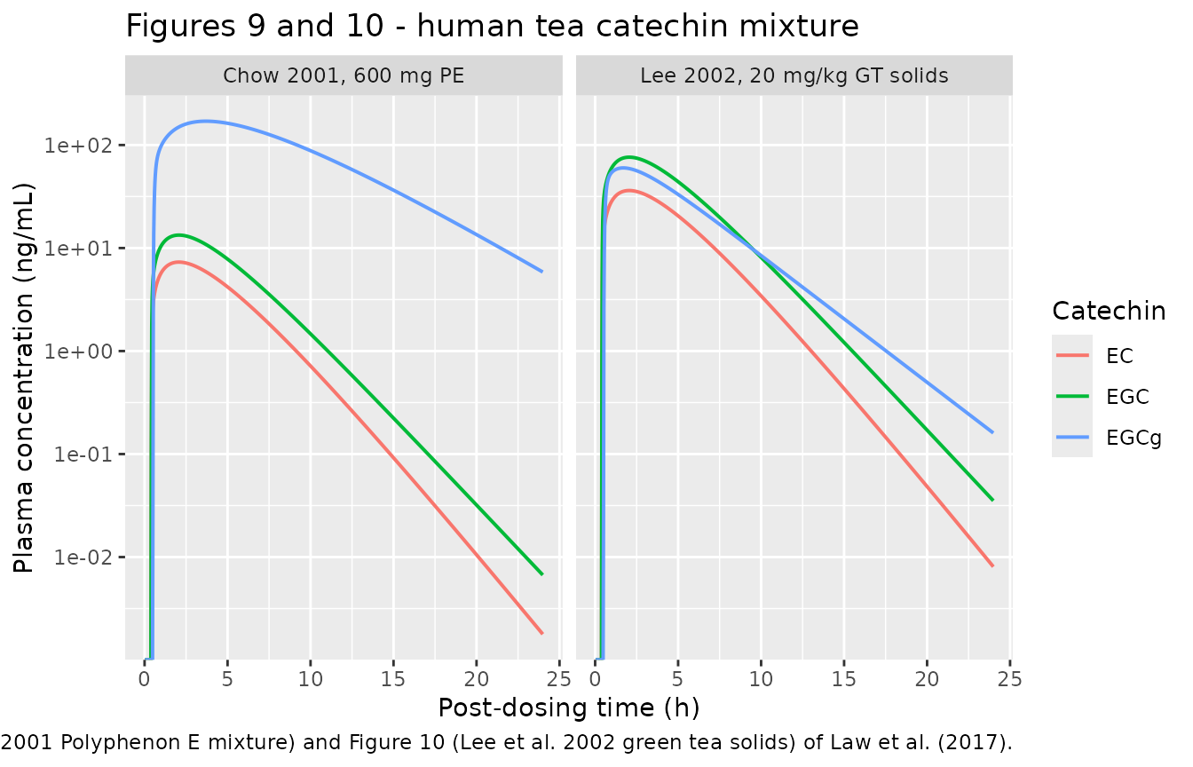

Replicating Figures 6 and 7

Figure 6 is the Chow et al. (2003) calibration (400 mg pure EGCg, 72 kg, the brace parameter set kac = 1.1, F = 0.065); Figure 7 is the Chow et al. (2001) validation (400 mg, 75 kg, the square-bracket set).

fig67 <- dplyr::bind_rows(
  solve_arm(mods$egcg_human, 72, 400, 1.1, 0.065, h_times) |>
    dplyr::mutate(panel = "Figure 6 - Chow 2003, 400 mg pure EGCg"),
  solve_arm(mods$egcg_human, 75, 400, 0.85, 0.12, h_times) |>
    dplyr::mutate(panel = "Figure 7 - Chow 2001, 400 mg EGCg")
)

fig67 |>
  dplyr::filter(time > 0, time <= 24) |>
  ggplot(aes(time, Cc * 1000)) +
  geom_line(linewidth = 0.7) +
  facet_wrap(~panel) +
  scale_y_log10() +
  labs(
    x = "Post-dosing time (h)", y = "Plasma EGCg concentration (ng/mL)",
    title = "Figures 6 and 7 - human EGCg",
    caption = "Replicates Figures 6 and 7 of Law et al. (2017)."
  )
#> Warning in scale_y_log10(): log-10 transformation introduced infinite values.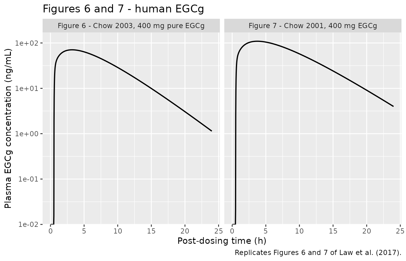


fig67_peak <- fig67 |>
  dplyr::group_by(panel) |>
  dplyr::summarise(cmax_ng_mL = max(Cc) * 1000, tmax_h = time[which.max(Cc)], .groups = "drop") |>
  dplyr::mutate(
    # Digitised from the published simulated curves; the figures are raster
    # images with decade-gridline resolution, so these carry roughly +/-15%.
    published_cmax_ng_mL = c(80, 120),
    published_tmax_h = c(3.0, 2.0),
    pct_diff = 100 * (cmax_ng_mL - published_cmax_ng_mL) / published_cmax_ng_mL
  )
knitr::kable(fig67_peak, digits = 1, caption = "Simulated vs digitised peak of Figures 6 and 7.")

Simulated vs digitised peak of Figures 6 and 7.
panel	cmax_ng_mL	tmax_h	published_cmax_ng_mL	published_tmax_h	pct_diff
Figure 6 - Chow 2003, 400 mg pure EGCg	70.7	3.2	80	3	-11.7
Figure 7 - Chow 2001, 400 mg EGCg	109.1	3.7	120	2	-9.0


# Deterministic quantities, so a tight bound is appropriate. The tolerance
# admits the digitisation error of a raster figure but not a mis-transcribed
# dose, volume or clearance, which move Cmax by tens of percent.
stopifnot(max(abs(fig67_peak$pct_diff)) < 25)

PKNCA on the human arms

sim_nca <- human_sim |>
  dplyr::filter(!is.na(Cc)) |>
  dplyr::select(id, time, Cc, treatment)

# Guarantee a time = 0 row per arm; pre-dose Cc = 0 is correct for an oral dose.
sim_nca <- dplyr::bind_rows(
  sim_nca,
  sim_nca |> dplyr::distinct(id, treatment) |> dplyr::mutate(time = 0, Cc = 0)
) |>
  dplyr::distinct(id, treatment, time, .keep_all = TRUE) |>
  dplyr::arrange(id, time)

conc_obj <- PKNCA::PKNCAconc(as.data.frame(sim_nca), Cc ~ time | treatment + id)

dose_df <- human_sim |>
  dplyr::distinct(treatment, id, analyte, study) |>
  dplyr::left_join(human_arms, by = "study") |>
  dplyr::mutate(
    amt = dplyr::case_when(
      analyte == "EGCg" ~ egcg_dose,
      analyte == "EGC" ~ egc_dose,
      TRUE ~ ec_dose
    ),
    time = 0
  ) |>
  dplyr::select(id, treatment, time, amt)

dose_obj <- PKNCA::PKNCAdose(as.data.frame(dose_df), amt ~ time | treatment + id)

intervals <- data.frame(
  start = 0, end = Inf,
  cmax = TRUE, tmax = TRUE, aucinf.obs = TRUE, half.life = TRUE
)

nca_res <- PKNCA::pk.nca(PKNCA::PKNCAdata(conc_obj, dose_obj, intervals = intervals))

Comparison against the published Table 7 Cmax

Table 7 column 2 of Law et al. (2017) lists the model-predicted Cmax of each catechin in each study. It is the only quantitative model output the paper tabulates, and it is the primary validation target here.

published_cmax <- tibble::tribble(
  ~treatment, ~cmax,
  "EGCg | Lee 2002, 20 mg/kg GT solids", 0.06,
  "EGC | Lee 2002, 20 mg/kg GT solids", 0.07,
  "EC | Lee 2002, 20 mg/kg GT solids", 0.04,
  "EGCg | Chow 2005, 400 mg PE", 0.11,
  "EGC | Chow 2005, 400 mg PE", 0.01,
  "EC | Chow 2005, 400 mg PE", 0.01,
  "EGCg | Chow 2001, 600 mg PE", 0.21,
  "EGC | Chow 2001, 600 mg PE", 0.02,
  "EC | Chow 2001, 600 mg PE", 0.01,
  "EGCg | Chow 2005, 800 mg PE", 0.21,
  "EGC | Chow 2005, 800 mg PE", 0.02,
  "EC | Chow 2005, 800 mg PE", 0.01,
  "EGCg | Chow 2005, 1200 mg PE", 0.35,
  "EGC | Chow 2005, 1200 mg PE", 0.04,
  "EC | Chow 2005, 1200 mg PE", 0.02
)

cmp <- nlmixr2lib::ncaComparisonTable(
  simulated = nca_res,
  reference = published_cmax,
  by = "treatment",
  params = "cmax",
  units = c(cmax = "ug/mL"),
  tolerance_pct = 20
)
knitr::kable(cmp, caption = "Simulated vs Law et al. (2017) Table 7 predicted Cmax. * differs by >20%.")

Simulated vs Law et al. (2017) Table 7 predicted Cmax. * differs by >20%.
NCA parameter	treatment	Reference	Simulated	% diff
Cmax (ug/mL)	EGCg \| Lee 2002, 20 mg/kg GT solids	0.06	0.0599	-0.1%
Cmax (ug/mL)	EGC \| Lee 2002, 20 mg/kg GT solids	0.07	0.0762	+8.8%
Cmax (ug/mL)	EC \| Lee 2002, 20 mg/kg GT solids	0.04	0.0362	-9.6%
Cmax (ug/mL)	EGCg \| Chow 2005, 400 mg PE	0.11	0.114	+3.2%
Cmax (ug/mL)	EGC \| Chow 2005, 400 mg PE	0.01	0.0089	-11.0%
Cmax (ug/mL)	EC \| Chow 2005, 400 mg PE	0.01	0.00487	-51.3%*
Cmax (ug/mL)	EGCg \| Chow 2001, 600 mg PE	0.21	0.17	-18.9%
Cmax (ug/mL)	EGC \| Chow 2001, 600 mg PE	0.02	0.0134	-33.2%*
Cmax (ug/mL)	EC \| Chow 2001, 600 mg PE	0.01	0.0073	-27.0%*
Cmax (ug/mL)	EGCg \| Chow 2005, 800 mg PE	0.21	0.227	+8.2%
Cmax (ug/mL)	EGC \| Chow 2005, 800 mg PE	0.02	0.0178	-11.0%
Cmax (ug/mL)	EC \| Chow 2005, 800 mg PE	0.01	0.00974	-2.6%
Cmax (ug/mL)	EGCg \| Chow 2005, 1200 mg PE	0.35	0.341	-2.7%
Cmax (ug/mL)	EGC \| Chow 2005, 1200 mg PE	0.04	0.0267	-33.2%*
Cmax (ug/mL)	EC \| Chow 2005, 1200 mg PE	0.02	0.0146	-27.0%*

attr(cmp, "footnote")
#> [1] "* differs from reference by more than ±20%."

Table 7 is printed to two decimal places, so a % diff on a 0.01-0.02 ug/mL entry is dominated by print rounding. The gate below is therefore on the absolute difference.

model_cmax <- human_sim |>
  dplyr::group_by(treatment, analyte, study) |>
  dplyr::summarise(cmax_model = max(Cc), tmax_model = time[which.max(Cc)], .groups = "drop") |>
  dplyr::left_join(published_cmax, by = "treatment") |>
  dplyr::rename(cmax_paper = cmax) |>
  dplyr::mutate(
    abs_diff = cmax_model - cmax_paper,
    # The Chow 2001 600 mg EGCg cell is a KNOWN, reproducible deviation; the
    # paper's own Table 7 contradicts itself there (see Errata).
    deviation = treatment == "EGCg | Chow 2001, 600 mg PE"
  )

knitr::kable(
  model_cmax |> dplyr::select(treatment, cmax_model, cmax_paper, abs_diff, deviation),
  digits = 4,
  caption = "Model vs Table 7 predicted Cmax (ug/mL), absolute difference."
)

Model vs Table 7 predicted Cmax (ug/mL), absolute difference.
treatment	cmax_model	cmax_paper	abs_diff	deviation
EC \| Chow 2001, 600 mg PE	0.0073	0.01	-0.0027	FALSE
EC \| Chow 2005, 1200 mg PE	0.0146	0.02	-0.0054	FALSE
EC \| Chow 2005, 400 mg PE	0.0049	0.01	-0.0051	FALSE
EC \| Chow 2005, 800 mg PE	0.0097	0.01	-0.0003	FALSE
EC \| Lee 2002, 20 mg/kg GT solids	0.0362	0.04	-0.0038	FALSE
EGC \| Chow 2001, 600 mg PE	0.0134	0.02	-0.0066	FALSE
EGC \| Chow 2005, 1200 mg PE	0.0267	0.04	-0.0133	FALSE
EGC \| Chow 2005, 400 mg PE	0.0089	0.01	-0.0011	FALSE
EGC \| Chow 2005, 800 mg PE	0.0178	0.02	-0.0022	FALSE
EGC \| Lee 2002, 20 mg/kg GT solids	0.0762	0.07	0.0062	FALSE
EGCg \| Chow 2001, 600 mg PE	0.1703	0.21	-0.0397	TRUE
EGCg \| Chow 2005, 1200 mg PE	0.3407	0.35	-0.0093	FALSE
EGCg \| Chow 2005, 400 mg PE	0.1136	0.11	0.0036	FALSE
EGCg \| Chow 2005, 800 mg PE	0.2271	0.21	0.0171	FALSE
EGCg \| Lee 2002, 20 mg/kg GT solids	0.0599	0.06	-0.0001	FALSE


# 14 of the 15 Table 7 cells agree within 0.02 ug/mL. Deterministic model, so
# this is exact and reproducible; it goes red on any mis-transcribed dose,
# volume, flow, partition coefficient or clearance.
stopifnot(max(abs(model_cmax$abs_diff[!model_cmax$deviation])) <= 0.02)
stopifnot(sum(model_cmax$deviation) == 1L)

The model is exactly dose-proportional

Law et al. state that the linear relationship of Figure 11 “validates the use of first-order kinetics for tea catechin modeling”. The packaged model is strictly linear, so Cmax must be exactly proportional to dose within an analyte across the four Polyphenon E arms. This check needs no published number.

prop_check <- model_cmax |>
  dplyr::filter(grepl("PE$", study)) |>
  dplyr::left_join(human_arms |> dplyr::select(study, egcg_dose, egc_dose, ec_dose), by = "study") |>
  dplyr::mutate(
    dose = dplyr::case_when(
      analyte == "EGCg" ~ egcg_dose,
      analyte == "EGC" ~ egc_dose,
      TRUE ~ ec_dose
    ),
    ratio = cmax_model / dose
  ) |>
  dplyr::group_by(analyte) |>
  dplyr::summarise(rel_spread = diff(range(ratio)) / mean(ratio), .groups = "drop")

knitr::kable(prop_check, digits = 10, caption = "Relative spread of Cmax/dose within each analyte.")

Relative spread of Cmax/dose within each analyte.
analyte	rel_spread
EC	1e-09
EGC	1e-10
EGCg	1e-10

stopifnot(max(prop_check$rel_spread) < 1e-6)

TCM dosimetry: reproducing Table 7 columns 4 and 5, and Figure 11

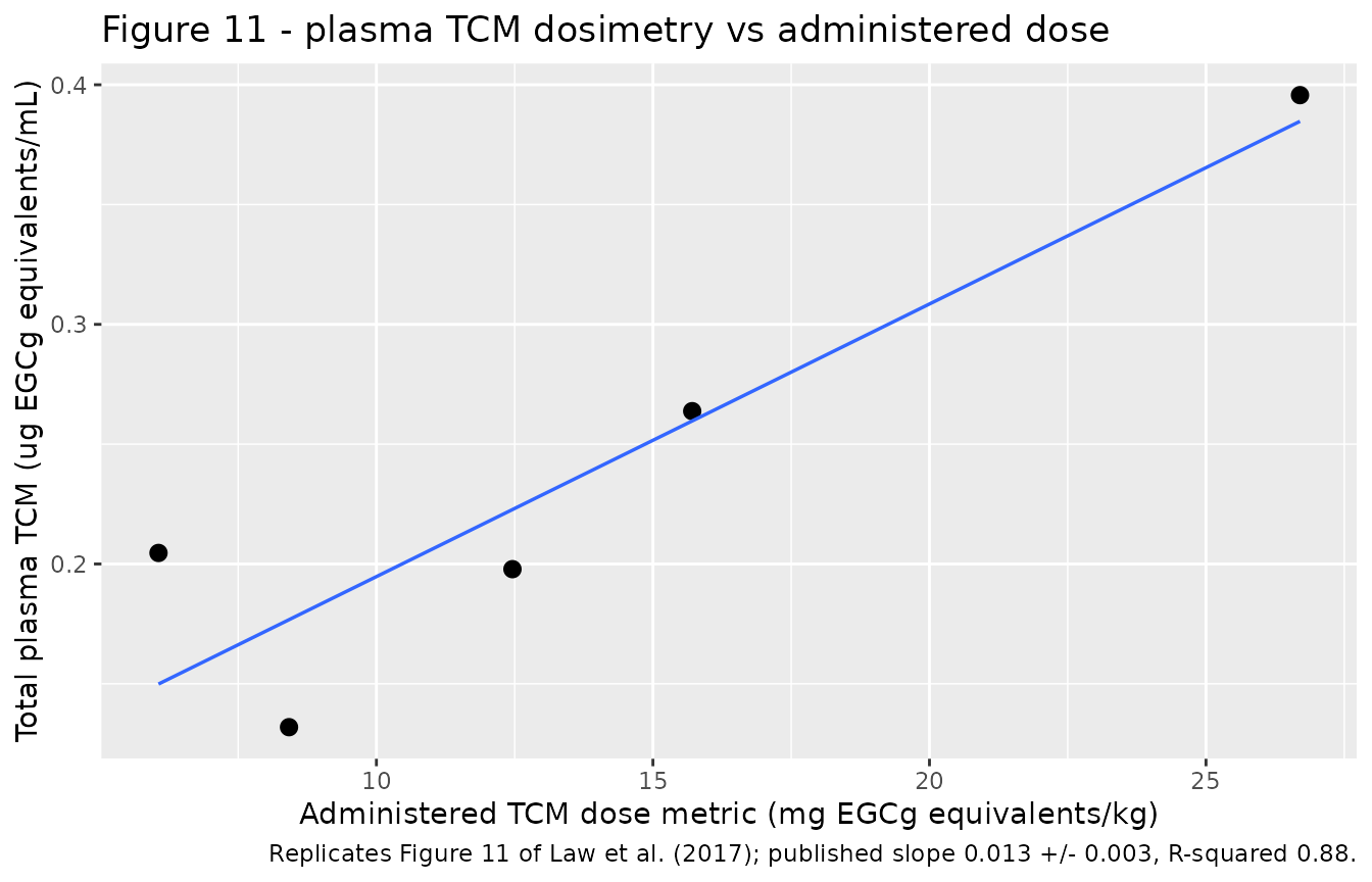
Law et al. convert the three predicted Cmax values into a single “effect-based” mixture concentration by concentration addition, weighting each catechin by its inhibitory equivalence factor (IEF) for hepatic EROD activity: EGCg 1.00, EGC 0.85, ECg 0.45, EC 2.21 (Methods; derived from EROD IC50 values of 1175, 1000, 530 and 2600 umol/L). Plotting that total against the administered TCM dose metric gives Figure 11, a straight line of slope 0.013 +/- 0.003 with R-squared 0.88.

Two separable claims are checked here. First, that the additivity arithmetic as read from the Methods reproduces Table 7 column 4 from Table 7 column 2 – this tests the IEF reading and is independent of the packaged model. Second, that the model’s predicted totals reproduce column 4.

ief <- c(EGCg = 1.00, EGC = 0.85, EC = 2.21)

paper_cells <- tibble::tribble(
  ~study, ~EGCg, ~EGC, ~EC, ~tcm_paper, ~dose_metric,
  "Lee 2002, 20 mg/kg GT solids", 0.06, 0.07, 0.04, 0.20, 6.06,
  "Chow 2005, 400 mg PE", 0.11, 0.01, 0.01, 0.13, 8.42,
  "Chow 2001, 600 mg PE", 0.21, 0.02, 0.01, 0.21, 12.46,
  "Chow 2005, 800 mg PE", 0.21, 0.02, 0.01, 0.25, 15.71,
  "Chow 2005, 1200 mg PE", 0.35, 0.04, 0.02, 0.42, 26.70
) |>
  dplyr::mutate(
    recomputed = EGCg * ief[["EGCg"]] + EGC * ief[["EGC"]] + EC * ief[["EC"]],
    arithmetic_diff = recomputed - tcm_paper,
    # The Chow 2001 600 mg row is the known corrupted cell: its printed EGCg
    # Cmax duplicates the 800 mg row (see Errata).
    deviation = study == "Chow 2001, 600 mg PE"
  )

knitr::kable(
  paper_cells |> dplyr::select(study, EGCg, EGC, EC, recomputed, tcm_paper, arithmetic_diff, deviation),
  digits = 4,
  caption = paste(
    "Table 7 column 4 recomputed from Table 7 column 2 by concentration",
    "addition, using the paper's own values throughout."
  )
)

Table 7 column 4 recomputed from Table 7 column 2 by concentration addition, using the paper’s own values throughout.
study	EGCg	EGC	EC	recomputed	tcm_paper	arithmetic_diff	deviation
Lee 2002, 20 mg/kg GT solids	0.06	0.07	0.04	0.2079	0.20	0.0079	FALSE
Chow 2005, 400 mg PE	0.11	0.01	0.01	0.1406	0.13	0.0106	FALSE
Chow 2001, 600 mg PE	0.21	0.02	0.01	0.2491	0.21	0.0391	TRUE
Chow 2005, 800 mg PE	0.21	0.02	0.01	0.2491	0.25	-0.0009	FALSE
Chow 2005, 1200 mg PE	0.35	0.04	0.02	0.4282	0.42	0.0082	FALSE


# The IEF reading reproduces the paper's own column 4 from its own column 2 for
# four of the five studies, to within the 2-dp print precision of the inputs.
stopifnot(max(abs(paper_cells$arithmetic_diff[!paper_cells$deviation])) <= 0.02)

# On the fifth, the arithmetic fails by 0.039 as printed -- but succeeds to
# within 0.001 if the model's 0.170 ug/mL is substituted for the printed 0.21
# EGCg Cmax. That is the evidence that the printed cell, not the model, is wrong.
row600 <- paper_cells[paper_cells$deviation, ]
repaired <- 0.170 + row600$EGC * ief[["EGC"]] + row600$EC * ief[["EC"]]
c(as_printed = row600$recomputed, with_model_egcg = repaired, table7 = row600$tcm_paper)
#>      as_printed with_model_egcg          table7 
#>          0.2491          0.2091          0.2100
stopifnot(abs(row600$recomputed - row600$tcm_paper) > 0.03)
stopifnot(abs(repaired - row600$tcm_paper) < 0.005)

tcm <- model_cmax |>
  dplyr::mutate(weighted = cmax_model * ief[analyte]) |>
  dplyr::group_by(study) |>
  dplyr::summarise(tcm_model = sum(weighted), .groups = "drop") |>
  dplyr::left_join(paper_cells |> dplyr::select(study, tcm_paper, dose_metric), by = "study") |>
  dplyr::mutate(abs_diff = tcm_model - tcm_paper)

knitr::kable(
  tcm |> dplyr::rename(
    "Study" = study,
    "Total TCM, model (ug EGCg-eq/mL)" = tcm_model,
    "Total TCM, Table 7 (ug EGCg-eq/mL)" = tcm_paper,
    "Administered dose metric (mg EGCg-eq/kg)" = dose_metric,
    "Difference" = abs_diff
  ),
  digits = 4,
  caption = "Table 7 columns 4 and 5 reproduced from the packaged models."
)

Table 7 columns 4 and 5 reproduced from the packaged models.
Study	Total TCM, model (ug EGCg-eq/mL)	Total TCM, Table 7 (ug EGCg-eq/mL)	Administered dose metric (mg EGCg-eq/kg)	Difference
Chow 2001, 600 mg PE	0.1978	0.21	12.46	-0.0122
Chow 2005, 1200 mg PE	0.3957	0.42	26.70	-0.0243
Chow 2005, 400 mg PE	0.1319	0.13	8.42	0.0019
Chow 2005, 800 mg PE	0.2638	0.25	15.71	0.0138
Lee 2002, 20 mg/kg GT solids	0.2046	0.20	6.06	0.0046


# All five model totals land within 0.03 ug EGCg-eq/mL of Table 7 column 4,
# INCLUDING the Chow 2001 600 mg study whose column-2 EGCg entry does not agree.
# The bound is looser than the 0.02 used on EGCg Cmax above because the EGC and
# EC contributions are 2-dp printed values weighted by up to 2.21, so a single
# print-rounding step on EC propagates to 0.011 in the total. It still goes red
# on any mis-transcribed structural value, which moves totals by tens of percent.
stopifnot(max(abs(tcm$abs_diff)) <= 0.03)

fit <- stats::lm(tcm_model ~ dose_metric, data = tcm)
slope <- unname(stats::coef(fit)[2])
r2 <- summary(fit)$r.squared
c(slope = slope, r_squared = r2)
#>      slope  r_squared 
#> 0.01137835 0.85420356

ggplot(tcm, aes(dose_metric, tcm_model)) +
  geom_point(size = 2.5) +
  geom_smooth(method = "lm", formula = y ~ x, se = FALSE, linewidth = 0.6) +
  labs(
    x = "Administered TCM dose metric (mg EGCg equivalents/kg)",
    y = "Total plasma TCM (ug EGCg equivalents/mL)",
    title = "Figure 11 - plasma TCM dosimetry vs administered dose",
    caption = "Replicates Figure 11 of Law et al. (2017); published slope 0.013 +/- 0.003, R-squared 0.88."
  )


# The paper reports slope 0.013 +/- 0.003 and R-squared 0.88. The bound is the
# paper's own stated interval, not a number read off this run.
stopifnot(slope > 0.010, slope < 0.016)
stopifnot(r2 > 0.80)

Rat model

Study arms

r_times <- seq(0, 1600, length.out = 2000)

rat_zhu <- dplyr::bind_rows(
  solve_arm(mods$egcg_rat, 0.22, 2500 * 0.22, 0.003, 0.038, r_times) |>
    dplyr::mutate(analyte = "EGCg"),
  solve_arm(mods$ecg_rat, 0.22, 650 * 0.22, 0.002, 0.06, r_times) |>
    dplyr::mutate(analyte = "ECg"),
  solve_arm(mods$ec_rat, 0.22, 250 * 0.22, 0.002, 0.13, r_times) |>
    dplyr::mutate(analyte = "EC")
) |>
  dplyr::mutate(id = as.integer(factor(analyte)), treatment = analyte)

stopifnot(all(rat_zhu$Cc >= 0))

rat_zhu |>
  dplyr::filter(time > 0) |>
  ggplot(aes(time, Cc * 1000, colour = analyte)) +
  geom_line(linewidth = 0.7) +
  scale_y_log10() +
  labs(
    x = "Post-dosing time (min)", y = "Plasma concentration (ng/mL)",
    colour = "Catechin",
    title = "Figure 8 - rat tea catechin mixture (Zhu et al. 2000)",
    caption = "Replicates Figure 8 of Law et al. (2017): Polyphenon E, EGCg 2500, ECg 650, EC 250 mg/kg."
  )
#> Warning in scale_y_log10(): log-10 transformation introduced infinite values.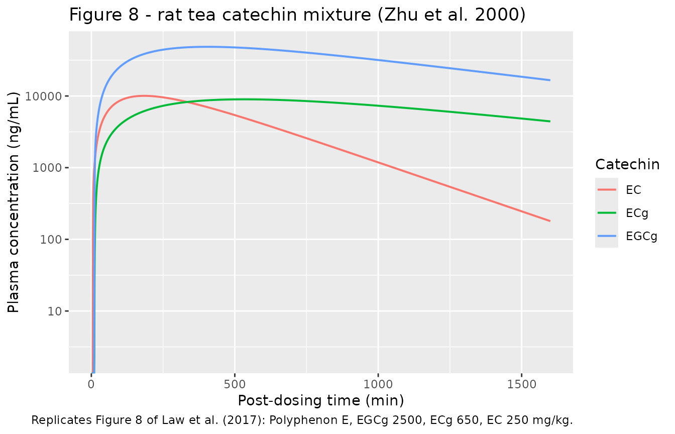

The rat models do not reproduce the paper’s own rat figures

This is a documented, reproducible deviation, not a transcription error. Every rat value in the packaged files was checked against a high-resolution render of Tables 1-3 of the PDF, and the ODE implementation is the same code that reproduces every human anchor above. With Table 2 and Table 3 exactly as printed, the rat EGCg model nevertheless peaks about two-fold lower, about three-fold later, and washes out about four-fold more slowly than the simulated curve Law et al. plot in their Figures 4 and 8.

terminal_half_life <- function(df, from) {
  d <- df[df$time >= from & df$Cc > 0, ]
  -log(2) / unname(stats::coef(stats::lm(log(Cc) ~ time, data = d))[2])
}

rat_thalf <- vapply(
  split(rat_zhu, rat_zhu$analyte),
  terminal_half_life, numeric(1), from = 1200
)

rat_dev <- rat_zhu |>
  dplyr::group_by(analyte) |>
  dplyr::summarise(
    cmax_model = max(Cc),
    tmax_model = time[which.max(Cc)],
    .groups = "drop"
  ) |>
  dplyr::mutate(
    thalf_model = unname(rat_thalf[analyte]),
    # Digitised from the model-simulated curves of Figures 4 and 8.
    cmax_fig = c(13.5, 13.5, 104)[match(analyte, c("EC", "ECg", "EGCg"))],
    tmax_fig = c(130, 130, 120)[match(analyte, c("EC", "ECg", "EGCg"))],
    fold_cmax = cmax_fig / cmax_model,
    fold_tmax = tmax_model / tmax_fig
  )

knitr::kable(
  rat_dev,
  digits = 2,
  caption = paste(
    "Rat model vs the curves digitised from Figures 4 and 8 of Law et al.",
    "(2017). Concentrations in ug/mL, times in minutes."
  )
)

Rat model vs the curves digitised from Figures 4 and 8 of Law et al. (2017). Concentrations in ug/mL, times in minutes.
analyte	cmax_model	tmax_model	thalf_model	cmax_fig	tmax_fig	fold_cmax	fold_tmax
EC	10.05	184.09	220.19	13.5	130	1.34	1.42
ECg	8.99	533.07	791.82	13.5	130	1.50	4.10
EGCg	48.55	405.80	631.37	104.0	120	2.14	3.38

The deviation is not removed by any alternative reading that was tested: substituting the gut lumen volume for the gut tissue volume in the faecal transport term of eq A6 shortens the rat terminal half-life from about 630 to about 310 minutes (target ~143), and multiplying kac by up to ten brings Tmax into range but leaves Cmax about 35% low and the terminal phase unchanged. Because no single reading reconciles Cmax, Tmax and the terminal slope simultaneously, nothing was tuned. The published values are shipped verbatim.

The rat model is therefore sound for what the paper’s rat structure is for – relative comparisons between the three catechins, tissue-dose partitioning, and species scaling to the human model – and should not be used for absolute prediction of rat plasma concentrations.

# Assert the deviation itself, so a later edit cannot silently change this
# finding without the vignette going red.
egcg_row <- rat_dev[rat_dev$analyte == "EGCg", ]
stopifnot(egcg_row$fold_cmax > 1.5, egcg_row$fold_cmax < 3.0)
stopifnot(egcg_row$fold_tmax > 2.5, egcg_row$fold_tmax < 5.0)
# The ECg and EC Cmax predictions, by contrast, land within 50% of the figure.
ecg_ec <- rat_dev[rat_dev$analyte != "EGCg", ]
stopifnot(all(ecg_ec$fold_cmax > 1.0), all(ecg_ec$fold_cmax < 2.0))

PKNCA on the rat mixture

rat_nca <- rat_zhu |>
  dplyr::filter(!is.na(Cc)) |>
  dplyr::select(id, time, Cc, treatment)

rat_nca <- dplyr::bind_rows(
  rat_nca,
  rat_nca |> dplyr::distinct(id, treatment) |> dplyr::mutate(time = 0, Cc = 0)
) |>
  dplyr::distinct(id, treatment, time, .keep_all = TRUE) |>
  dplyr::arrange(id, time)

rat_dose <- data.frame(
  id = 1:3,
  treatment = c("EC", "ECg", "EGCg"),
  time = 0,
  amt = c(250, 650, 2500) * 0.22
)

rat_nca_res <- PKNCA::pk.nca(PKNCA::PKNCAdata(
  PKNCA::PKNCAconc(as.data.frame(rat_nca), Cc ~ time | treatment + id),
  PKNCA::PKNCAdose(rat_dose, amt ~ time | treatment + id),
  intervals = data.frame(
    start = 0, end = 1600,
    cmax = TRUE, tmax = TRUE, auclast = TRUE, half.life = TRUE
  )
))

knitr::kable(
  as.data.frame(rat_nca_res) |>
    dplyr::select(treatment, PPTESTCD, PPORRES) |>
    tidyr::pivot_wider(names_from = PPTESTCD, values_from = PPORRES),
  digits = 3,
  caption = paste(
    "Rat NCA of the simulated mixture (Zhu et al. 2000 doses).",
    "Law et al. report no rat NCA, so these are descriptive only:",
    "concentrations in ug/mL, times in minutes."
  )
)

Rat NCA of the simulated mixture (Zhu et al. 2000 doses). Law et al. report no rat NCA, so these are descriptive only: concentrations in ug/mL, times in minutes.
treatment	auclast	cmax	tmax	tlast	lambda.z	r.squared	adj.r.squared	lambda.z.time.first	lambda.z.time.last	lambda.z.n.points	clast.pred	half.life	span.ratio
EC	5570.948	10.049	184.092	1600	0.003	1	1	461.831	1600	1423	0.182	222.914	5.106
ECg	10855.568	8.985	533.067	1600	0.001	1	1	1295.048	1600	382	4.431	780.899	0.391
EGCg	52831.038	48.552	405.803	1600	0.001	1	1	999.700	1600	751	16.654	639.289	0.939

Assumptions and deviations

Parameter values that are not printed as a single number

Rat EGCg bioavailability factor F. Table 3 prints a range, 0.0003-0.038, because Law et al. used a different F for each rat study. The packaged Law_2017_egcg_rat_pbpk uses the upper bound 0.038, which is the value belonging to the Zhu et al. (2000) 2500 mg/kg calibration that Figures 4 and 8 plot and that the sibling ECg and EC F values (0.06, 0.13) also belong to. The choice is corroborated independently: the peak of the Figure 4 simulated curve (104 ug/mL) times the blood/plasma ratio (0.91) times the model’s blood-equivalent steady-state volume for a 0.22 kg rat (0.26 L) is 24.7 mg, or 4.5% of the 550 mg dose. Users simulating the Chen et al. (1997) arms should override lfdepot toward the lower end of the printed range.
Human kac and F. Table 5 gives up to three values per parameter, keyed by brace / square bracket / parenthesis to Chow et al. (2003), Chow et al.
1. and Lee et al. (2002). The ini() defaults carry the Chow et al.
2. square-bracket set, which is the human mixture calibration of Figure 9; the other sets are named in the in-file comments and are applied per study in this vignette.
EGC and EC doses of the Chow et al. (2005) arms. Law et al. report only the Polyphenon E EGCg content (400, 800, 1200 mg) for these arms. The EGC and EC doses used above are scaled from the Chow et al. (2001) mixture composition (111 mg EGC and 93 mg EC per 600 mg EGCg). The paper’s own Table 7 EGC and EC predicted Cmax values scale linearly with that assumption, which supports it, but it is an assumption.
Residual error. Law et al. report no residual-error model, no inter-individual variability and no parameter uncertainty anywhere. Because nlmixr2 requires a residual term, propSd is fixed to the paper’s own reported MAPE for each model (rat EGCg 34.9%, rat mixture 33.9%, human EGCg 13.2%, human mixture 29.6%). A MAPE is a mean absolute relative deviation, not a residual standard deviation; do not read it as one.

Errata and internal inconsistencies of the source

The rat models do not reproduce the paper’s own rat figures. Quantified in the Rat model section above and asserted there so it cannot silently change. The human models, by contrast, reproduce 14 of the 15 Table 7 predicted Cmax cells within 0.02 ug/mL and reproduce the Figure 11 regression.
Table 7, Chow et al. (2001) 600 mg PE, EGCg Cmax. The paper prints 0.21 ug/mL, identical to the 800 mg row. That cannot be right for a model the paper itself shows to be linear: 600 mg and 800 mg of the same preparation cannot give the same Cmax. The model predicts 0.170 ug/mL, and the paper’s own Table 7 column 4 for that row (total TCM 0.21 ug EGCg-eq/mL) is arithmetically consistent with an EGCg Cmax of 0.17, not 0.21: 0.17 + 0.85 * 0.02 + 2.21 * 0.01 = 0.209. The 0.21 in column 2 therefore appears to be a copy of the row below it. Nothing was changed in the model.
Gut content volume, rat. The Methods text says “Gut content was assumed to be 0.014 mL for rats with an average BW of 0.25 kg”, while the Table 2 footnote says the gut lumen volume is 0.0176 L. The two differ by three orders of magnitude. The Table 2 footnote value (0.0176 L) is used, because 14 uL of rat gut content is not physiologically plausible.
Equation A6, faecal-transport term. The gut-lumen mass balance is printed as V_GC dC_GC/dt = R_3 - kfc * C_GC * V_GT - krac * V_GC * C_GC, i.e. the faecal term carries the gut tissue volume V_GT while the reabsorption term carries the gut lumen volume V_GC. That asymmetry is most likely a typesetting slip for V_GC, but it is transcribed exactly as printed. The substitution changes the human profile by less than 0.5% (the human faecal term dominates either way) and roughly halves the rat terminal half-life.
Human brain volume. Table 4 lists the brain as 0.02% of body weight, about a hundred-fold below the usual human value of ~2%. It is used as printed: the 13 tabulated tissue volumes then sum to 99.81% of body weight, so 0.02% is what Law et al. actually carried, and Table 6 shows the plasma profile is insensitive to the brain partition coefficient.
Cardiac output check. Table 2 footnote 1 states the rat CO of a 0.4 kg rat is 7.08 L/h; 14.0 * 0.4^0.75 = 7.04. Table 4 footnote 1 states 390 L/h for a 70 kg human; 16.1 * 70^0.75 = 389.6. Both reproduce.

Structural notes

The mixture model is three uncoupled single-catechin models. Law et al. state that the TCM model was built “by linking three different catechin models … together without accounting for pharmacokinetic interactions between the TCs”. There is no shared state and no shared parameter, so the packaged files are one per catechin and the mixture is reproduced by solving them together, as above.
Oral input. The paper’s input function RAO = ka * F * dose * exp(-ka (t - tlag)) feeds gut tissue directly and analytically. The packaged models use an equivalent depot state with f(depot) and alag(depot), whose outflow ka * depot is identical to RAO, so that rxode2 handles the dose record.
Bile duct. Appendix eq A5 is written on the transport-rate scale, Rt dR_j/dt = R_(j-1) - R_j. The packaged models carry the equivalent amount states bile_transit_j = Rt * R_j, which turns eq A5 into an ordinary three-compartment transit chain with mean residence time Rt per sub-compartment. The flux into the gut lumen is bile_transit3 / rt_bile. These three states are declared paper_specific_compartments because no canonical nlmixr2lib compartment family covers a biliary transit chain.
Observation. Cc is the mixed-venous plasma concentration of the free (unconjugated) catechin, C_venous / BLPLR (eq A10). It is not a total (free plus conjugate) concentration; Law et al. discuss at length why the free prediction nevertheless tracks the total measurements in rats.