Fenebrutinib popPK and ACR / DAS28 exposure-response (Chan 2020)
Source:vignettes/articles/Chan_2020_fenebrutinib.Rmd
Chan_2020_fenebrutinib.RmdModel and source
Chan 2020 reports three linked analyses of fenebrutinib (GDC-0853), a noncovalent Bruton’s tyrosine kinase inhibitor, in rheumatoid arthritis (RA). Each is packaged as its own model:
-
Chan_2020_fenebrutinib: the population PK model (Model S1, Table I). -
Chan_2020_fenebrutinib_acr: the longitudinal logistic exposure-response (E-R) model for ACR20 / ACR50 / ACR70 (Model S2, Table S4). -
Chan_2020_fenebrutinib_das28: the longitudinal E-R model for DAS28 (CRP) (Model S3, Table S5).
Both E-R models are driven by the individual steady-state daily AUC
that the popPK model predicts, supplied as the covariate column
AUC_FENEBRUTINIB. The paper’s fourth analysis, a
model-based meta-analysis (Data S1), prints only its R start values and
no final estimates, so it is not packaged.
- Citation: Chan P, Yu J, Chinn L, Prohn M, Huisman J, Matzuka B, Hanley W, Tuckwell K, Quartino A. Population Pharmacokinetics, Efficacy Exposure-response Analysis, and Model-based Meta-analysis of Fenebrutinib in Subjects with Rheumatoid Arthritis. Pharm Res. 2020;37(2):25. doi:10.1007/s11095-019-2752-y. (A correction notice revised only the article title; no parameter value is affected.)
- Article: https://doi.org/10.1007/s11095-019-2752-y (open access; supplement ESM 1 holds Tables S1-S5 and the NONMEM control streams)
mod_pk <- rxode2::rxode2(readModelDb("Chan_2020_fenebrutinib"))
#> ℹ parameter labels from comments will be replaced by 'label()'
#> Warning: some etas defaulted to non-mu referenced, possible parsing error: etaiov_f_1, etaiov_f_2, etaiov_f_3, etaiov_f_4, etaiov_f_5
#> as a work-around try putting the mu-referenced expression on a simple line
mod_acr <- rxode2::rxode2(readModelDb("Chan_2020_fenebrutinib_acr"))
#> ℹ parameter labels from comments will be replaced by 'label()'
mod_das <- rxode2::rxode2(readModelDb("Chan_2020_fenebrutinib_das28"))
#> ℹ parameter labels from comments will be replaced by 'label()'
Population
The popPK analysis pooled 385 subjects (Table S2): 78 healthy volunteers from two phase 1 studies (GA29347 multiple ascending dose, powder-in-capsule; GP29832 relative bioavailability / food / rabeprazole interaction) and 307 adults with moderate to severe RA from the phase 2 ANDES trial (GA29350), who took 50 mg QD, 150 mg QD or 200 mg BID tablets for 12 weeks. Pooled age was 18-75 years (median 48), weight 38-153 kg (median 73), and 66.2% were female. In phase 2, 99.3% of patients were classified as fed and 39.7% took a proton-pump inhibitor (PPI).
The two E-R analyses used the 467 phase 2 patients of the placebo and fenebrutinib arms of cohorts 1 (MTX-IR) and 2 (TNF-IR) (Table S3): median age 52, 81% female, enrolled in Eastern Europe (62%), Latin America (33%) and the US (5%). ACR responses were recorded on days 7, 14, 28, 56 and 84 (non-responder imputation); DAS28 (CRP) on days 0, 7, 14, 28, 56 and 84 (LOCF).
The same information is available programmatically through each
model’s population metadata,
e.g. readModelDb("Chan_2020_fenebrutinib")()$population.
Source trace
Every ini() value carries an in-file comment naming its
source. They are collected here.
PopPK model (Model S1, Table I)
Table I prints every log-transformed THETA back-transformed, so the
packaged log-scale values are log() of the printed
numbers.
| Parameter | Value | Source |
|---|---|---|
lcl |
log(19.5 L/h) | Table I, theta1 |
lvc |
log(381 L) | Table I, theta2 |
lvp |
log(284 L) | Table I, theta3 |
lq |
log(52.8 L/h) | Table I, theta4 |
lvp2 |
log(273 L) | Table I, theta5 |
lq2 |
log(4.47 L/h) | Table I, theta6 |
lnn (NTR) |
log(14.9) | Table I, theta7 |
lmtt (MTT) |
log(0.849 h) | Table I, theta8 |
lfdepot |
log(1), fixed | Model S1 TVF1 = 1
|
e_fed_mtt |
log(1.43) | Table I, theta11 |
e_conmed_ppi_mtt |
log(0.835) | Table I, theta12 |
e_ppi_fed_mtt |
log(2.26) | Table I, theta13 |
e_conmed_ppi_f |
log(0.657) | Table I, theta14 |
e_ppi_fed_f |
log(0.693) | Table I, theta15 |
e_fed_nn |
log(0.864) | Table I, theta16 |
e_tablet_nn |
log(0.049) | Table I, theta17 |
e_conmed_ppi_cl |
log(0.663) | Table I, theta20 |
e_age_cl |
-0.161 | Table I, theta22 (untransformed, RSE 41.4%) |
e_healthy_cl |
log(1.52) | Table I, theta23 |
etalcl, etalvc, etalmtt,
etalfdepot
|
0.0732, 0.100, 0.0861, 0.131 | Table I, omega1.1, 2.2, 8.8, 9.9 |
etaiov_f_1 … etaiov_f_5
|
0.299 | Table I, omega10.1 ($OMEGA BLOCK(1) SAME for occasions
2-5) |
propSd (patients) |
0.390 | Table I, theta21 |
propSd_hv |
1.94 | Table I, theta9 |
lkruv_hv |
log(1.94 1/h) | Table I, theta18 |
logitfruv_hv |
log(6.66) | Table I, theta19
(ERRMAX = EXP(THETA(19))/(1+EXP(THETA(19)))) |
| CL covariate model | exp((AGE/48)^theta22) * exp(HV*theta23) * exp(PPI*theta20) |
Model S1 CLAGE, CLCOV,
CL
|
| Savic transit input |
exp(log(DOS*F1) + NTR*log(KTR*t) + log(KTR) - KTR*t - logNTR!),
KTR = (NTR+1)/MTT
|
Model S1 $DES INP1, KTR1,
LOGF1 (Stirling) |
| Residual error | proportional; HV:
exp(theta9) * (1 - ERRMAX*(1 - exp(-exp(theta18)*TAD)))
|
Model S1 $ERROR
|
ACR20 / ACR50 / ACR70 E-R model (Model S2, Table S4)
| Parameter | Value | Source |
|---|---|---|
logit_bl_acr20 / _acr50 /
_acr70
|
-4.62 / -6.47 / -8.3 | Table S4, theta1-3 |
e_pdv_acr (Markov) |
0.934 | Table S4, theta4 |
emax_pbo_acr |
3.41 | Table S4, theta7 |
lt50_pbo_acr20 |
log(21.5 d) | Table S4, theta8 (EXP(TVLET50) in Model S2) |
lt50_pbo_acr5070 |
log(32.8 d) | Table S4, theta11 |
lhill_pbo_acr |
log(2.52) | Table S4, theta12 (HILL = EXP(THETA(12))) |
emax_acr |
1.39 | Table S4, theta9 (Eastern Europe) |
lec50_acr |
log(2650 h*ng/mL) | Table S4, theta10 |
e_region_usa_emax_acr |
2.13 | Table S4, theta13 (REGCOV) |
e_region_latam_emax_acr |
2.06 | Table S4, theta14 |
etalogit_bl_acr |
4.85 | Table S4, omega16.1 |
| Logit | base_k + Emax_pbo*t^h/(t^h + T50_k^h) + Emax*REGCOV*AUC/(AUC + EC50) + theta4*PDV + eta |
Model S2 LOGIT
|
DAS28 (CRP) E-R model (Model S3, Table S5)
| Parameter | Value | Source |
|---|---|---|
lrbase_das28 |
log(5.46) | Table S5, theta1 (C = TVC*EXP(ETA(1))) |
emax_pbo_das28 |
-1.36 | Table S5, theta2 |
lt50_pbo_das28 |
log(36.7 d) | Table S5, theta3 (used when DOSE = 0) |
lt50_das28 |
log(47 d) | Table S5, theta4 (used when DOSE > 0) |
lec50_das28 |
log(293 h*ng/mL) | Table S5, theta5 |
emax_das28 |
-0.964 | Table S5, theta6 |
etalrbase_das28, etaemax_das28
|
0.0206, 0.283 | Table S5, omega1.1, omega2.2 |
addSd_das28 |
0.3 | Table S5, sigma |
| Time course | C + (theta2 + theta6*AUC/(EAUC50 + AUC))*exp(eta2) * t/(t + T50) |
Model S3 $PRED (THILL = 1) |
Population PK
Covariate effects on CL/F
The Results quote three covariate contrasts on CL/F. The PPI and healthy-volunteer effects are single THETAs and reproduce exactly. The age contrast is evaluated from the exponent as printed.
age_fac <- function(age) exp((age / 48)^-0.161)
cov_check <- data.frame(
  Contrast = c(
    "PPI co-medication vs none",
    "Healthy volunteer vs RA patient",
    "Age 75 vs 25 years"
  ),
  Published = c("-33.7%", "+52%", "-15.2%"),
  Model = sprintf("%+.1f%%", 100 * (c(0.663, 1.52, age_fac(75) / age_fac(25)) - 1))
)
knitr::kable(cov_check)| Contrast | Published | Model |
|---|---|---|
| PPI co-medication vs none | -33.7% | -33.7% |
| Healthy volunteer vs RA patient | +52% | +52.0% |
| Age 75 vs 25 years | -15.2% | -16.5% |
The age contrast from the printed equation is -16.5%, 1.3 percentage
points from the published -15.2%. A plain power model
(AGE/48)^-0.161 gives -16.2%, so neither form reproduces
-15.2% exactly (see Assumptions and deviations).
Healthy-volunteer profile (phase 1)
The Introduction reports, for the phase 1 multiple ascending dose study in healthy volunteers (powder-in-capsule, fasted), a Tmax of 1-3 h and a steady-state half-life of 4.2-9.9 h. Typical-value profiles for a 35-year-old healthy volunteer (GA29347 median) after 14 days of dosing:
mod_pk_typ <- rxode2::zeroRe(mod_pk)
#> Warning: No sigma parameters in the model
#> Warning: some etas defaulted to non-mu referenced, possible parsing error: etaiov_f_1, etaiov_f_2, etaiov_f_3, etaiov_f_4, etaiov_f_5
#> as a work-around try putting the mu-referenced expression on a simple line
make_pk_events <- function(id, dose, ii, ndays, obs_times) {
  n_dose <- ndays * 24 / ii
  dose_rows <- data.frame(
    id = id, time = (seq_len(n_dose) - 1) * ii, amt = dose, evid = 1L, cmt = "central"
  )
  obs_rows <- data.frame(id = id, time = obs_times, amt = 0, evid = 0L, cmt = "central")
  dplyr::bind_rows(dose_rows, obs_rows) |> dplyr::arrange(time, dplyr::desc(evid))
}
hv_regimens <- data.frame(
  id = 1:4,
  regimen = c("60 mg BID", "150 mg BID", "250 mg BID", "500 mg QD"),
  dose = c(60, 150, 250, 500),
  ii = c(12, 12, 12, 24)
)
last_dose <- 13 * 24 # morning dose of day 14
ev_hv <- do.call(rbind, lapply(seq_len(nrow(hv_regimens)), function(i) {
  r <- hv_regimens[i, ]
  make_pk_events(r$id, r$dose, r$ii, 14, last_dose + seq(0, 48, by = 0.1))
})) |>
  mutate(
    AGE = 35, DIS_HEALTHY = 1, CONMED_PPI = 0, FED = 0,
    FORM_FENEBRUTINIB_TABLET = 0, OCC = 0
  )
# The BID regimens continue to an evening dose; drop it so the 48 h after the
# last morning dose describe the washout, as in GA29347's day-14 sampling.
ev_hv <- ev_hv |> filter(!(evid == 1 & time > 13 * 24))
sim_hv <- rxode2::rxSolve(mod_pk_typ, events = ev_hv, returnType = "data.frame") |>
  left_join(hv_regimens, by = "id")
#> ℹ omega/sigma items treated as zero: 'etalcl', 'etalvc', 'etalmtt', 'etalfdepot', 'etaiov_f_1', 'etaiov_f_2', 'etaiov_f_3', 'etaiov_f_4', 'etaiov_f_5'
#> Warning: multi-subject simulation without without 'omega'

loglin_thalf <- function(t, conc, from, to) {
  k <- t >= from & t <= to
  log(2) / -coef(lm(log(conc[k]) ~ t[k]))[[2]]
}
hv_nca <- sim_hv |>
  mutate(tad = time - 13 * 24) |>
  group_by(regimen) |>
  summarise(
    tmax = tad[which.max(Cc)],
    thalf_2_12 = loglin_thalf(tad, Cc, 2, 12),
    thalf_4_24 = loglin_thalf(tad, Cc, 4, 24),
    thalf_12_24 = loglin_thalf(tad, Cc, 12, 24),
    thalf_24_48 = loglin_thalf(tad, Cc, 24, 48),
    .groups = "drop"
  )
hv_nca |>
  dplyr::rename(
    "Regimen" = regimen, "Tmax (h)" = tmax,
    "t1/2, 2-12 h" = thalf_2_12, "t1/2, 4-24 h" = thalf_4_24,
    "t1/2, 12-24 h" = thalf_12_24, "t1/2, 24-48 h" = thalf_24_48
  ) |>
knitr::kable(digits = 1, caption = "Typical healthy-volunteer Tmax and log-linear half-life (h) by fitting window after the last day-14 dose.")| Regimen | Tmax (h) | t1/2, 2-12 h | t1/2, 4-24 h | t1/2, 12-24 h | t1/2, 24-48 h |
|---|---|---|---|---|---|
| 150 mg BID | 1.3 | 4.4 | 7.3 | 8.8 | 13.3 |
| 250 mg BID | 1.3 | 4.4 | 7.3 | 8.8 | 13.3 |
| 500 mg QD | 1.3 | 3.9 | 6.7 | 8.3 | 11.9 |
| 60 mg BID | 1.3 | 4.4 | 7.3 | 8.8 | 13.3 |
A three-compartment disposition has no single half-life: the log-linear slope lengthens from about 4 h (2-12 h after the dose) to about 13 h (24-48 h), as the slow third phase (Q2/F = 4.47 L/h, V3/F = 273 L) takes over. The published 4.2-9.9 h is a range of individual NCA values whose fitting window is not stated. Over the dosing interval (4-24 h) the typical value sits in the middle of that range, which is the gate below; the 24-48 h slope is longer than any published value.
stopifnot(
  all(hv_nca$tmax >= 1 & hv_nca$tmax <= 3),
  all(hv_nca$thalf_4_24 >= 4.2 & hv_nca$thalf_4_24 <= 9.9)
)
ggplot(sim_hv |> mutate(tad = time - 13 * 24), aes(tad, Cc, colour = regimen)) +
  geom_line() +
  scale_y_log10() +
  labs(x = "Time after last dose (h)", y = "Fenebrutinib (ng/mL)", colour = NULL) +
  theme_bw()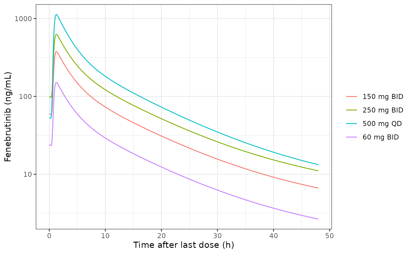
Typical healthy-volunteer concentration after the last day-14 morning dose (powder-in-capsule, fasted).
Phase 2 virtual cohort and steady-state AUC (Figure S3)
A virtual phase 2 cohort of 200 patients per fenebrutinib arm: all fed (99.3% in Table S2), 39.7% PPI co-medicated, tablet formulation, age drawn from a normal distribution with the phase 2 mean and SD (50.6, 12 years) truncated to 19-75 years. The model is solved stochastically for 14 days (steady state is reached within a few days), and the daily AUC(0-24) on day 14 is computed with PKNCA. The E-R analyses used exactly this quantity, the individual post hoc steady-state daily AUC at the nominal dose.
set.seed(2752)
n_per_arm <- 200
arms <- data.frame(
  treatment = c("50 mg QD", "150 mg QD", "200 mg BID"),
  dose = c(50, 150, 200),
  ii = c(24, 24, 12)
)
cohort <- do.call(rbind, lapply(seq_len(nrow(arms)), function(i) {
  data.frame(
    id = (i - 1) * n_per_arm + seq_len(n_per_arm),
    treatment = arms$treatment[i],
    dose = arms$dose[i],
    ii = arms$ii[i]
  )
}))
draw_age <- function(n) {
  x <- rnorm(n * 3, 50.6, 12)
  x <- x[x >= 19 & x <= 75]
  x[seq_len(n)]
}
cohort$AGE <- draw_age(nrow(cohort))
cohort$CONMED_PPI <- rbinom(nrow(cohort), 1, 0.397)

obs_day14 <- 13 * 24 + c(0, 0.5, 1, 1.5, 2, 3, 4, 6, 8, 10, 12, 12.5, 13, 13.5, 14, 15, 16, 18, 20, 22, 24)
ev_p2 <- do.call(rbind, lapply(seq_len(nrow(cohort)), function(i) {
  make_pk_events(cohort$id[i], cohort$dose[i], cohort$ii[i], 14, obs_day14)
})) |>
  left_join(cohort |> select(id, treatment, AGE, CONMED_PPI), by = "id") |>
  mutate(DIS_HEALTHY = 0, FED = 1, FORM_FENEBRUTINIB_TABLET = 1, OCC = 0)

rxode2::rxSetSeed(2752)
sim_p2 <- rxode2::rxSolve(
  mod_pk,
  events = ev_p2,
  keep = c("treatment", "CONMED_PPI"),
  returnType = "data.frame"
)
conc_p2 <- sim_p2 |>
  filter(!is.na(Cc)) |>
  select(id, time, Cc, treatment)
dose_p2 <- ev_p2 |>
  filter(evid == 1) |>
  select(id, time, amt, treatment)
o_conc <- PKNCA::PKNCAconc(conc_p2, Cc ~ time | treatment + id)
o_dose <- PKNCA::PKNCAdose(dose_p2, amt ~ time | treatment + id)
intervals <- data.frame(start = 13 * 24, end = 14 * 24, auclast = TRUE, cmax = TRUE)
nca_p2 <- PKNCA::pk.nca(PKNCA::PKNCAdata(o_conc, o_dose, intervals = intervals))
auc_ind <- as.data.frame(nca_p2$result) |>
  filter(PPTESTCD == "auclast") |>
  select(id, treatment, AUC = PPORRES)
# Figure S3 digitised: black dot = median, box = interquartile range.
figS3 <- data.frame(
  treatment = arms$treatment,
  median = c(1170, 3370, 7000),
  q25 = c(740, 2400, 4300),
  q75 = c(2100, 5150, 10400)
)
auc_summary <- auc_ind |>
  group_by(treatment) |>
  summarise(
    sim_median = median(AUC),
    sim_q25 = quantile(AUC, 0.25),
    sim_q75 = quantile(AUC, 0.75),
    .groups = "drop"
  ) |>
  left_join(figS3, by = "treatment") |>
  mutate(pct_diff_median = 100 * (sim_median / median - 1)) |>
  arrange(match(treatment, arms$treatment))
auc_summary |>
  dplyr::rename(
    "Arm" = treatment,
    "Simulated median" = sim_median,
    "Simulated Q1" = sim_q25,
    "Simulated Q3" = sim_q75,
    "Figure S3 median" = median,
    "Figure S3 Q1" = q25,
    "Figure S3 Q3" = q75,
    "Median difference (%)" = pct_diff_median
  ) |>
knitr::kable(digits = 0, caption = "Steady-state daily AUC (h*ng/mL): simulation vs Figure S3 of Chan 2020.")| Arm | Simulated median | Simulated Q1 | Simulated Q3 | Figure S3 median | Figure S3 Q1 | Figure S3 Q3 | Median difference (%) |
|---|---|---|---|---|---|---|---|
| 50 mg QD | 819 | 594 | 1154 | 1170 | 740 | 2100 | -30 |
| 150 mg QD | 2370 | 1754 | 3102 | 3370 | 2400 | 5150 | -30 |
| 200 mg BID | 6723 | 4703 | 9868 | 7000 | 4300 | 10400 | -4 |
pct <- setNames(auc_summary$pct_diff_median, auc_summary$treatment)
# Figure S3 plots post hoc EBEs, which shrink toward the typical value, so the
# centre is the gate, not the spread. A mis-transcribed CL/F, F1 or unit (or
# dropping the e-scaling of CL/F, which inflates AUC 2.7-fold) moves every
# median by far more than these bounds.
stopifnot(
  # 200 mg BID, the arm carrying most of the E-R data, reproduces.
  abs(pct[["200 mg BID"]]) < 15,
  # Known deviation, see below: the QD arms sit about 30% under Figure S3.
  # The bound fixes the direction and size of that gap instead of hiding it.
  all(pct[c("50 mg QD", "150 mg QD")] > -45 & pct[c("50 mg QD", "150 mg QD")] < 0)
)
Deviation: the QD arms. The model is linear, so its dose-normalised steady-state AUC is the same for every regimen (about 16-17 hng/mL per daily mg in this cohort). Figure S3 is not dose-proportional: its medians give 23.4 (50 mg QD), 22.5 (150 mg QD) and 17.5 (200 mg BID) hng/mL per daily mg. No parameter set of the published structure can reproduce all three, and this vignette does not tune. The 200 mg BID arm matches; the two QD arms come out about 30% low. A plausible cause is that the phase 2 EBEs of the QD patients (sparse trough sampling, 27-58% eta shrinkage) carry information the typical covariate model does not, but the paper does not discuss it.
ggplot(auc_ind, aes(AUC, factor(treatment, levels = arms$treatment))) +
  geom_boxplot(outlier.shape = 1) +
  geom_point(data = figS3, aes(median, treatment), shape = 4, size = 3, colour = "red") +
  labs(x = "AUC(0-24) at steady state (h*ng/mL)", y = NULL) +
  theme_bw()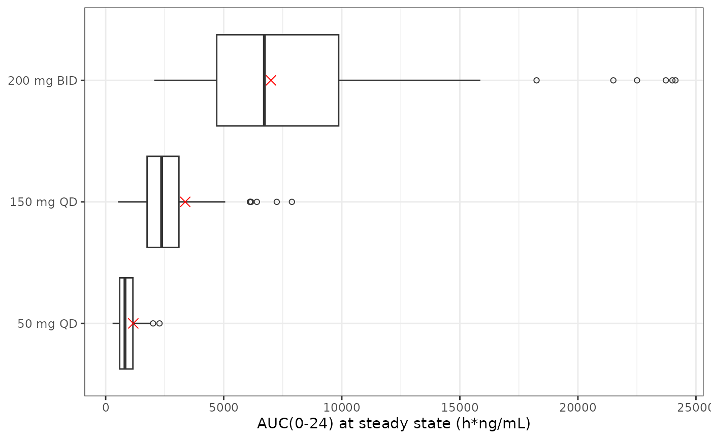
Replicates Figure S3 of Chan 2020: distribution of the individual steady-state daily AUC by dose group. Crosses mark the Figure S3 medians.
NCA comparison against the published exposure
The paper reports no NCA table; its only exposure numbers are the
Figure S3 medians, which are compared here with
ncaComparisonTable() (it pools the per-arm simulated values
by their median).
nlmixr2lib::ncaComparisonTable(
  simulated = nca_p2,
  reference = figS3 |> transmute(treatment, auclast = median),
  by = "treatment",
  params = "auclast",
  units = c(auclast = "h*ng/mL"),
  tolerance_pct = 30
) |>
knitr::kable(caption = "Simulated vs Figure S3 median AUC0-24 at steady state.")| NCA parameter | treatment | Reference | Simulated | % diff |
|---|---|---|---|---|
| AUClast (h*ng/mL) | 50 mg QD | 1170 | 819 | -30.0%* |
| AUClast (h*ng/mL) | 150 mg QD | 3370 | 2370 | -29.7% |
| AUClast (h*ng/mL) | 200 mg BID | 7000 | 6720 | -4.0% |
ACR20 / ACR50 / ACR70 exposure-response
Virtual E-R cohort
Each fenebrutinib patient keeps the AUC simulated above; a placebo
arm of 200 patients has AUC_FENEBRUTINIB = 0. Region is
drawn with the Table S3 proportions (Eastern Europe 62%, Latin America
33%, US 5%).
The model contains a Markov term on the previous visit’s response
(PDV), so responses are simulated visit by visit: every
patient is evaluated at each visit with PDV = 0 and with
PDV = 1, and a Bernoulli chain then picks the probability
that matches the patient’s own previous simulated response
(PDV = 0 at day 7, because every patient is a non-responder
at baseline). The subject-level random effect is drawn in R and supplied
as a data column, so the cohort does not depend on rxode2’s
thread-partitioned RNG.
set.seed(20200106)
er_cohort <- bind_rows(
  data.frame(id = 1000 + seq_len(n_per_arm), treatment = "Placebo", AUC = 0),
  auc_ind |> select(id, treatment, AUC)
) |>
  mutate(
    region = sample(c("Eastern Europe", "Latin America", "US"), n(),
      replace = TRUE, prob = c(0.62, 0.33, 0.05)
    ),
    REGION_USA = as.integer(region == "US"),
    REGION_EASTEUROPE = as.integer(region == "Eastern Europe"),
    etalogit_bl_acr = rnorm(n(), 0, sqrt(4.85))
  )
acr_days <- c(7, 14, 28, 56, 84)
ev_acr <- tidyr::expand_grid(id = er_cohort$id, time = acr_days, PDV = c(0, 1)) |>
  left_join(er_cohort, by = "id") |>
  rename(AUC_FENEBRUTINIB = AUC) |>
  mutate(evid = 0L, amt = 0) |>
  arrange(id, time, PDV)
p_acr <- rxode2::rxSolve(
  rxode2::zeroRe(mod_acr),
  events = ev_acr,
  keep = c("treatment", "PDV"),
  returnType = "data.frame"
)
#> ℹ omega/sigma items treated as zero: 'etalogit_bl_acr'
#> Warning: multi-subject simulation without without 'omega'
# Structural check on the solve itself: with the Markov term, a previous
# responder always has the higher probability (logit shift theta4 = 0.934).
wide <- p_acr |>
  select(id, time, PDV, prob_acr20) |>
  tidyr::pivot_wider(names_from = PDV, values_from = prob_acr20, names_prefix = "p")
stopifnot(all(abs(qlogis(wide$p1) - qlogis(wide$p0) - 0.934) < 1e-6))
run_chain <- function(p0, p1) {
  # p0 / p1: probabilities at successive visits given PDV = 0 / PDV = 1
  y <- integer(length(p0))
  prev <- 0L
  for (k in seq_along(p0)) {
    p <- if (prev == 1L) p1[k] else p0[k]
    y[k] <- as.integer(stats::runif(1) < p)
    prev <- y[k]
  }
  y
}
set.seed(84)
acr_long <- p_acr |>
  select(id, treatment, time, PDV, prob_acr20, prob_acr50, prob_acr70) |>
  tidyr::pivot_longer(starts_with("prob_"), names_to = "endpoint", values_to = "p") |>
  mutate(endpoint = toupper(sub("prob_", "", endpoint))) |>
  tidyr::pivot_wider(names_from = PDV, values_from = p, names_prefix = "p") |>
  arrange(id, endpoint, time) |>
  group_by(id, endpoint) |>
  mutate(response = run_chain(p0, p1)) |>
  ungroup()
acr_frac <- acr_long |>
  group_by(treatment, endpoint, time) |>
  summarise(fraction = mean(response), .groups = "drop")
arm_levels <- c("Placebo", arms$treatment)
ggplot(acr_frac, aes(time, fraction, colour = endpoint)) +
  geom_line() +
  geom_point() +
  facet_wrap(~ factor(treatment, levels = arm_levels), nrow = 1) +
  labs(x = "Time (d since start of treatment)", y = "Fraction ACR responders", colour = NULL) +
  theme_bw()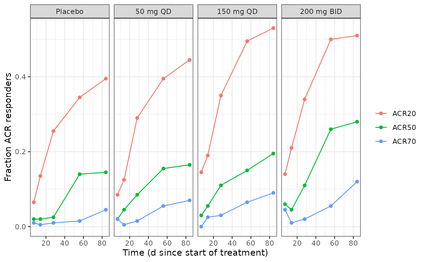
Replicates Figure 1 of Chan 2020: simulated fraction of ACR20 / ACR50 / ACR70 responders by visit and dose group.
Day-84 responder fractions against Figure 1
Figure 1 draws the median model prediction for each arm and threshold; the day-84 values are digitised below.
fig1_day84 <- tibble::tribble(
  ~treatment, ~endpoint, ~published,
  "Placebo", "ACR20", 0.37,
  "Placebo", "ACR50", 0.13,
  "Placebo", "ACR70", 0.03,
  "50 mg QD", "ACR20", 0.45,
  "50 mg QD", "ACR50", 0.30,
  "50 mg QD", "ACR70", 0.05,
  "150 mg QD", "ACR20", 0.53,
  "150 mg QD", "ACR50", 0.25,
  "150 mg QD", "ACR70", 0.09,
  "200 mg BID", "ACR20", 0.60,
  "200 mg BID", "ACR50", 0.31,
  "200 mg BID", "ACR70", 0.13
)
acr_cmp <- acr_frac |>
  filter(time == 84) |>
  inner_join(fig1_day84, by = c("treatment", "endpoint")) |>
  mutate(difference = fraction - published) |>
  arrange(match(treatment, arm_levels), endpoint)
acr_cmp |>
  select(treatment, endpoint, fraction, published, difference) |>
  dplyr::rename(
    "Arm" = treatment, "Endpoint" = endpoint, "Simulated" = fraction,
    "Figure 1 median prediction" = published, "Difference" = difference
  ) |>
knitr::kable(digits = 3, caption = "Day-84 fraction of responders.")| Arm | Endpoint | Simulated | Figure 1 median prediction | Difference |
|---|---|---|---|---|
| Placebo | ACR20 | 0.395 | 0.37 | 0.025 |
| Placebo | ACR50 | 0.145 | 0.13 | 0.015 |
| Placebo | ACR70 | 0.045 | 0.03 | 0.015 |
| 50 mg QD | ACR20 | 0.445 | 0.45 | -0.005 |
| 50 mg QD | ACR50 | 0.165 | 0.30 | -0.135 |
| 50 mg QD | ACR70 | 0.070 | 0.05 | 0.020 |
| 150 mg QD | ACR20 | 0.530 | 0.53 | 0.000 |
| 150 mg QD | ACR50 | 0.195 | 0.25 | -0.055 |
| 150 mg QD | ACR70 | 0.090 | 0.09 | 0.000 |
| 200 mg BID | ACR20 | 0.510 | 0.60 | -0.090 |
| 200 mg BID | ACR50 | 0.280 | 0.31 | -0.030 |
| 200 mg BID | ACR70 | 0.120 | 0.13 | -0.010 |
# 200 patients per arm give a binomial SE of about 0.035 at p = 0.5, and the
# huge logit IIV (omega^2 = 4.85) widens it further. Assert on the centre of
# the twelve differences and on a robust envelope, not on the worst cell.
stopifnot(
  abs(median(acr_cmp$difference)) < 0.05,
  quantile(abs(acr_cmp$difference), 0.9) < 0.12
)
DAS28 (CRP) exposure-response
The same E-R cohort (same AUC values) is carried through the DAS28 model. The two random effects are drawn in R, as for the ACR model.
set.seed(28)
das_cohort <- er_cohort |>
  select(id, treatment, AUC) |>
  mutate(
    etalrbase_das28 = rnorm(n(), 0, sqrt(0.0206)),
    etaemax_das28 = rnorm(n(), 0, sqrt(0.283))
  )
ev_das <- tidyr::expand_grid(id = das_cohort$id, time = c(0, 7, 14, 28, 56, 84)) |>
  left_join(das_cohort, by = "id") |>
  rename(AUC_FENEBRUTINIB = AUC) |>
  mutate(evid = 0L, amt = 0)
sim_das <- rxode2::rxSolve(
  rxode2::zeroRe(mod_das),
  events = ev_das,
  keep = "treatment",
  returnType = "data.frame"
)
#> ℹ omega/sigma items treated as zero: 'etalrbase_das28', 'etaemax_das28'
#> Warning: multi-subject simulation without without 'omega'
das_summary <- sim_das |>
  group_by(treatment, time) |>
  summarise(
    median = median(das28),
    lo = quantile(das28, 0.05),
    hi = quantile(das28, 0.95),
    .groups = "drop"
  )
ggplot(das_summary, aes(time, median)) +
  geom_ribbon(aes(ymin = lo, ymax = hi), fill = "salmon", alpha = 0.4) +
  geom_line(colour = "red") +
  facet_wrap(~ factor(treatment, levels = arm_levels), nrow = 1) +
  labs(x = "Time (d since start of treatment)", y = "DAS28 (CRP)") +
  theme_bw()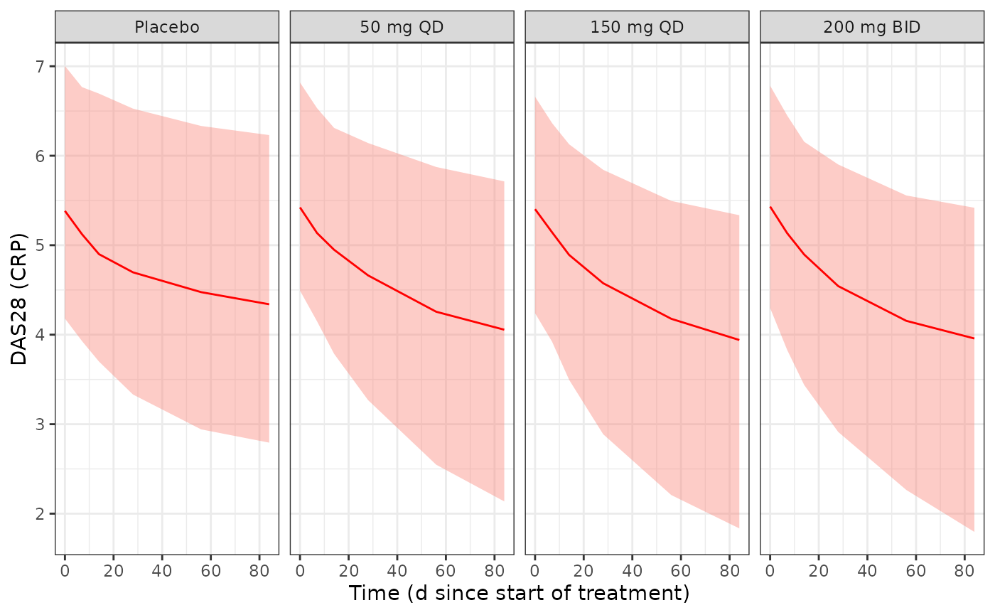
Replicates Figure 3 of Chan 2020: median and 90% interval of the model-predicted DAS28 (CRP) by dose group (residual error not added).
# Figure 3 median-prediction lines at day 84, digitised.
fig3_day84 <- data.frame(
  treatment = arm_levels,
  published = c(4.47, 3.97, 3.88, 3.85)
)
das_cmp <- das_summary |>
  filter(time == 84) |>
  inner_join(fig3_day84, by = "treatment") |>
  mutate(difference = median - published) |>
  arrange(match(treatment, arm_levels))
das_cmp |>
  select(treatment, median, published, difference) |>
  dplyr::rename(
    "Arm" = treatment, "Simulated median" = median,
    "Figure 3 median prediction" = published, "Difference" = difference
  ) |>
knitr::kable(digits = 2, caption = "Day-84 DAS28 (CRP).")| Arm | Simulated median | Figure 3 median prediction | Difference |
|---|---|---|---|
| Placebo | 4.34 | 4.47 | -0.13 |
| 50 mg QD | 4.06 | 3.97 | 0.09 |
| 150 mg QD | 3.94 | 3.88 | 0.06 |
| 200 mg BID | 3.96 | 3.85 | 0.11 |
baseline_median <- median(sim_das$das28[sim_das$time == 0])
stopifnot(
  abs(baseline_median - 5.46) < 0.1,
  all(abs(das_cmp$difference) < 0.2)
)
The drug arms’ medians sit below the typical-value prediction (for
200 mg BID, about 3.99 at the median AUC) because the random effect
multiplies the negative Emax through exp(eta), whose right
skew drags the median of the sum down. Figure 3 shows the same
offset.
Assumptions and deviations
-
Clearance scale. Model S1 multiplies CL by
EXP((AGE/48)**THETA(22)), which equals e = 2.718, not 1, at the reference age, so the 19.5 L/h of Table I is not the typical CL/F; a typical 48-year-old patient without PPI has CL/F = 53 L/h. The model reproduces the equation as printed. Dropping the e factor would raise every steady-state AUC 2.7-fold, far outside Figure S3, and would lengthen the healthy-volunteer half-life beyond the published 4.2-9.9 h. Both published numbers agree only with the e-scaled reading. - QD-arm exposure. The simulated steady-state AUC medians of the two QD arms are about 30% below Figure S3, while 200 mg BID matches. Figure S3 is less than dose-proportional, which a linear model cannot reproduce (see the Figure S3 section). The ACR and DAS28 simulations inherit the lower QD exposures, which is the most likely reason the 50 mg QD ACR50 fraction is the largest single miss against Figure 1.
- Age contrast. With the printed equation, CL/F is 16.5% lower at 75 than at 25 years, against the published 15.2%. The gap is too small to point to a different equation (a plain power model gives 16.2%) and is most likely rounding of THETA(22) (RSE 41.4%).
-
Coded but untabulated parameters, fixed at 0. Model
S1 codes an additive residual error THETA(10) and IIV on V2/F, Q1/F,
V3/F, Q2/F and NTR (ETA(3) to ETA(7)); Table I reports none of them and
the Results describe “a proportional error model”, so they are omitted.
The same applies to the rheumatoid-factor exponent THETA(15) of Model
S2. The Results call baseline RF “a statistically significant covariate”
and the schematic equation lists “Rheumatoid factor”, but Table S4 gives
no THETA(15) and the Discussion states “region was the only covariate in
the longitudinal E-R model”. The RF term is therefore omitted (exponent
0) and documented under
covariatesDataExcluded. The value was never published; the authors could confirm it. -
ACR model encoding. Model S2 is a
$PREDBernoulli likelihood with no residual error; the package encodes the three probabilities as outputsprob_acr20,prob_acr50,prob_acr70with a fixed placeholder additive error of 0.001 so that the model is a valid nlmixr2 object. Model S2 picks one threshold per record throughTYPE; the packaged model evaluates all three at once, andPDVmust be the previous response for the threshold being read. Table S4 labels the random effect “IOV on baseline”, but Model S2 has a single subject-level ETA, which is how it is encoded. -
Markov simulation. How the published posterior
predictive check handled
PDVis not stated. This vignette propagates each patient’s own simulated responses (a Bernoulli chain), which is the only self-contained choice. -
Occasion IOV. The phase 2 AUC simulation uses
OCC = 0(no IOV on F1), because the paper computed the E-R driver as a steady-state AUC at the nominal dose, not as an occasion-specific value. - E-R cohort composition. The virtual cohort gives every arm 200 patients and ignores the placebo/cohort-2 split and the correlation between region and AUC; the published Figures 1 and 3 use the observed patients (40 to about 150 per arm).
- Figure axis units. Figures 2 and 4 label their AUC axis “h.nM”, while Table S4, Table S5 and Figure S3 give ngh/mL, and the AUC values on Figures 2 and 4 span the same range as Figure S3. The packaged models use hng/mL, the unit printed next to both EC50 values.
- DAS28 residual error. Table S5 prints sigma = 0.3 (RSE 2.2%). An RSE of 2.2% is below the asymptotic floor of an estimated variance for 2676 observations (about 2.7%) but above the floor of an SD, and the table labels the omegas “omega2” but the sigma plain “sigma”, so 0.3 is used as the SD.
- Figure digitisation. Figure S3 medians and quartiles, Figure 1 day-84 median predictions and Figure 3 day-84 median predictions were read from the published images and carry reading error of about 0.01-0.02 in fraction, 0.03 in DAS28 score and 100-200 h*ng/mL in AUC.