Tegafur / 5-FU with Sipjeondaebo-tang in rats (Kim 2017)
Source:vignettes/articles/Kim_2017_tegafur_rat.Rmd
Kim_2017_tegafur_rat.RmdModel and source
- Citation: Kim TH, Shin S, Shin JC, Bulitta JB, Weon KY, Yoo SD, Park GY, Jeong SW, Kwon DR, Min BS, Woo MH, Shin BS. Effect of Sipjeondaebo-Tang on the Pharmacokinetics of S-1, an Anticancer Agent, in Rats Evaluated by Population Pharmacokinetic Modeling. Molecules. 2017;22(9):1488. doi:10.3390/molecules22091488
- Description: Preclinical (rat). Population PK model for oral tegafur (given as the fluoropyrimidine combination S-1) and its active metabolite 5-FU in male Sprague-Dawley rats, with a herb-drug interaction arm for the traditional Korean polyherbal medicine Sipjeondaebo-tang (SDT, 1200 mg/kg/day orally for seven consecutive days before the S-1 dose; Kim 2017). Tegafur is dosed into an absorption-site compartment that drains by two competing first-order routes: intact tegafur into a two-compartment tegafur disposition model (Ka), and pre-systemic first-pass metabolism in gut and liver into an amount-only pool of the 5-FU precursor 5’-hydroxytegafur (Ka,Met). The precursor pool is additionally fed systemically by the fraction FMet of tegafur clearance and converts to 5-FU at KConv; 5-FU then follows its own two-compartment disposition. SDT pretreatment is carried as the binary covariate CONMED_SDT, which selects between separately estimated control and SDT-pretreated values of Ka, Ka,Met and the 5-FU clearance; all other parameters are shared across the two arms. Repeated SDT dosing slowed tegafur absorption and raised 5-FU clearance 1.68-fold, reducing 5-FU exposure. Residual error is not reported in the source and is carried as fixed(0) – see vignette Errata.
- Article: https://doi.org/10.3390/molecules22091488 (open access, PMC6151713)
No supplementary material accompanies this article; every value below comes from the main text, Table 1 or Table 2.
Population
Kim 2017 studied male Sprague-Dawley rats (8 weeks, 280-300 g) at the Catholic University of Daegu (IACUC-2013-025). Rats were pretreated by oral gavage with either Sipjeondaebo-tang (SDT) 1200 mg/kg or the 1% CMC-Na vehicle, as a single dose or once daily for seven consecutive days (n = 5 per arm per schedule). One minute after the final pretreatment dose, S-1 was given orally as a mixture of tegafur 5 mg/kg, gimeracil 1.45 mg/kg and oteracil potassium 4.9 mg/kg in 7.5% DMSO. Plasma was sampled predose and at 0.25, 0.5, 1, 1.5, 2, 3, 4, 8, 12 and 24 h, and tegafur, 5-FU and gimeracil were assayed by LC/MS/MS (LLOQ 50, 10 and 50 ng/mL).
The population model (Section 4.5) was fitted to the tegafur and 5-FU profiles after oral S-1, together with a plasma 5-FU profile after intravenous 5-FU 10 mg/kg from an earlier study by the same group. Gimeracil was assayed and analysed noncompartmentally but is not part of the population model, so it is not represented in this model file; the gimeracil result is nevertheless the paper’s mechanistic explanation for the 5-FU effect.
The same information is available programmatically via
readModelDb("Kim_2017_tegafur_rat")()$population.
Model structure
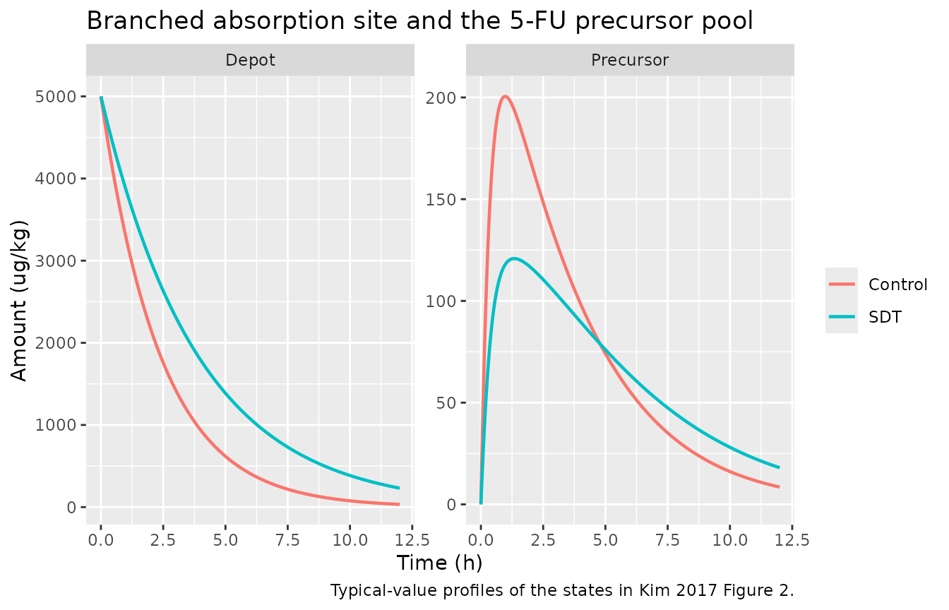
The model is a parent-metabolite cascade with a branched absorption site (Kim 2017 Figure 2 and equations 1-6). The dosing compartment drains by two competing first-order routes:
-
kacarries intact tegafur into a two-compartment tegafur disposition model; -
k_precursor_5fu_form(the paper’sKa,Met) represents first-pass metabolism in gut and liver, delivering drug directly into an amount-only pool of the 5-FU precursor 5’-hydroxytegafur.
The precursor pool is additionally fed systemically by the
fraction fm (the paper’s FMet) of tegafur
clearance, and converts to 5-FU at k_5fu_form
(KConv). 5-FU then follows its own two-compartment
disposition.
Because ka (0.296 1/h) is far below the tegafur
elimination rate constant cl/vc (0.0813 / 0.0464 = 1.75
1/h), tegafur is flip-flop: the terminal slope reflects
absorption, not elimination. The paper uses this to explain why the 5-FU
half-life (2.2-3.1 h) tracks tegafur’s rather than 5-FU’s own intrinsic
half-life of under 20 minutes.
SDT pretreatment enters as the binary covariate
CONMED_SDT, which selects between separately estimated
control and SDT values of ka,
k_precursor_5fu_form and cl_5fu. All other
parameters are shared.
Source trace
Every ini() entry carries an in-file comment naming its
source row; they are collected here for review.
| Equation / parameter | Value | Source location |
|---|---|---|
d/dt(depot) |
n/a | Kim 2017 equation 1 |
d/dt(central) |
n/a | Kim 2017 equation 2 |
d/dt(peripheral1) |
n/a | Kim 2017 equation 3 |
d/dt(precursor_5fu) |
n/a | Kim 2017 equation 4 |
d/dt(central_5fu) |
n/a | Kim 2017 equation 5 |
d/dt(peripheral1_5fu) |
n/a | Kim 2017 equation 6 |
lka_ctl (Ka,Con) |
0.296 1/h | Table 2 row 1 |
lka_sdt (Ka,Pretre) |
0.197 1/h | Table 2 row 2 |
lk_precursor_5fu_form_ctl (Ka,Met,Con) |
0.122 1/h | Table 2 row 3 |
lk_precursor_5fu_form_sdt (Ka,Met,Pretre) |
0.0595 1/h | Table 2 row 4 |
lk_5fu_form (KConv) |
2.88 1/h | Table 2 row 5 |
lcl (CLTeg/F) |
0.0813 L/h/kg | Table 2 row 6 |
fm (FMet) |
0.342 | Table 2 row 7 |
lcl_5fu_ctl (CL5FU,Con/F) |
3.52 L/h/kg | Table 2 row 8 |
lcl_5fu_sdt (CL5FU,Pretre/F) |
5.93 L/h/kg | Table 2 row 9 |
lq (CLdTeg/F) |
0.184 L/h/kg | Table 2 row 10 |
lq_5fu (CLd5FU/F) |
1.87 L/h/kg | Table 2 row 11 |
lvc (V1,Teg/F) |
0.0464 L/kg | Table 2 row 12 |
lvc_5fu (V1,5FU/F) |
0.623 L/kg | Table 2 row 13 |
lvp (V2,Teg/F) |
0.137 L/kg | Table 2 row 14 |
lvp_5fu (V2,5FU/F) |
0.294 L/kg | Table 2 row 15 |
All eta* variances |
see Table 2 | Table 2 parenthesised BSV column |
| Residual error | not published | Section 4.5 declares the structure only |
| Dose 5 mg/kg tegafur | 5000 ug/kg | Section 4.2 |
| Sampling schedule | 0-24 h | Section 4.2 |
Units
Amounts are carried in ug/kg and volumes in L/kg (the paper’s
clearances and volumes are body-weight normalised), so concentrations
come out in ug/L, which is numerically ng/mL – the unit Table 1 uses.
The tegafur dose of 5 mg/kg is therefore entered as
amt = 5000.
mod <- readModelDb("Kim_2017_tegafur_rat")
ui <- rxode2::rxode2(mod)
#> ℹ parameter labels from comments will be replaced by 'label()'
stopifnot(identical(ui$meta$units$concentration, "ng/mL"))
Virtual cohort
Original observed data are not public. Two arms of 200 virtual rats each are simulated at the paper’s actual sampling times, so the NCA below uses the same trapezoidal support the published analysis did.
# rxode2's RNG is partitioned per solver thread, so this cohort is not
# byte-identical across machines with different thread counts. Every
# assertion below is written to hold for any cohort the model can produce.
set.seed(20170907)
rxode2::rxSetSeed(20170907)

sample_times <- c(0, 0.25, 0.5, 1, 1.5, 2, 3, 4, 8, 12, 24)
n_per_arm <- 200L
tegafur_dose_ug_kg <- 5000

make_arm <- function(n, sdt, label, id_offset = 0L) {
  ids <- id_offset + seq_len(n)
  dosing <- tibble(
    id = ids, time = 0, amt = tegafur_dose_ug_kg,
    evid = 1L, cmt = "depot"
  )
  # Two endpoints are declared in the model, so observation rows must name
  # the OBSERVABLE (not the ODE state). Cc and Cc_5fu are both returned as
  # columns at every output row, so one set of rows serves both analytes.
  obs <- tidyr::expand_grid(id = ids, time = sample_times) |>
    mutate(amt = NA_real_, evid = 0L, cmt = "Cc")
  bind_rows(dosing, obs) |>
    mutate(CONMED_SDT = sdt, arm = label) |>
    arrange(id, time, desc(evid))
}

events <- bind_rows(
  make_arm(n_per_arm, 0, "Control", id_offset = 0L),
  make_arm(n_per_arm, 1, "SDT", id_offset = n_per_arm)
)

# Disjoint IDs across arms are mandatory: rxSolve keys subjects on id and
# would silently merge duplicates into one double-dosed subject.
stopifnot(!anyDuplicated(unique(events[, c("id", "time", "evid")])))
stopifnot(length(intersect(
  events$id[events$arm == "Control"], events$id[events$arm == "SDT"]
)) == 0)
Simulation
sim <- rxode2::rxSolve(mod, events = events, keep = c("arm", "CONMED_SDT")) |>
  as.data.frame()
#> ℹ parameter labels from comments will be replaced by 'label()'

# Residual error is fixed(0) in this model (not published), so Cc / Cc_5fu are
# the individual predictions; they are used directly rather than `sim`.
stopifnot(all(c("Cc", "Cc_5fu", "arm") %in% names(sim)))
A deterministic typical-value replication is used for the structural check against Table 1:
mod_typical <- rxode2::zeroRe(mod)
#> ℹ parameter labels from comments will be replaced by 'label()'
# Dense grid for the typical-value profiles used in the figures.
ev_typ_dense <- bind_rows(
  lapply(c(0, 1), function(sdt) {
    tibble(
      id = sdt + 1L,
      time = c(0, seq(0.02, 24, by = 0.02)),
      amt = NA_real_, evid = 0L, cmt = "Cc",
      CONMED_SDT = sdt, arm = if (sdt == 0) "Control" else "SDT"
    ) |>
      bind_rows(tibble(
        id = sdt + 1L, time = 0, amt = tegafur_dose_ug_kg,
        evid = 1L, cmt = "depot", CONMED_SDT = sdt,
        arm = if (sdt == 0) "Control" else "SDT"
      )) |>
      arrange(time, desc(evid))
  })
)

sim_typ <- rxode2::rxSolve(
  mod_typical, events = ev_typ_dense, keep = c("arm", "CONMED_SDT")
) |>
  as.data.frame()
#> ℹ omega/sigma items treated as zero: 'etalka_ctl', 'etalka_sdt', 'etalk_precursor_5fu_form_ctl', 'etalk_precursor_5fu_form_sdt', 'etalk_5fu_form', 'etalcl', 'etafm', 'etalcl_5fu_ctl', 'etalcl_5fu_sdt', 'etalq', 'etalq_5fu', 'etalvc', 'etalvc_5fu', 'etalvp', 'etalvp_5fu'
#> Warning: multi-subject simulation without without 'omega'
Replicate published figures
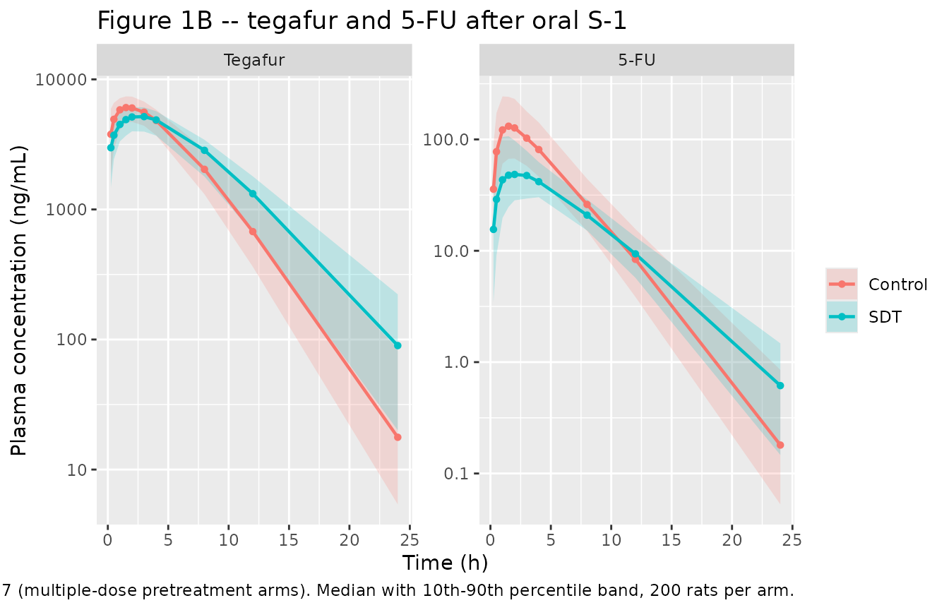
# Replicates Figure 1B of Kim 2017: mean plasma tegafur and 5-FU vs time after
# oral S-1, control vs seven-day SDT pretreatment.
sim |>
  select(id, time, arm, Tegafur = Cc, `5-FU` = Cc_5fu) |>
  pivot_longer(c(Tegafur, `5-FU`), names_to = "analyte", values_to = "conc") |>
  mutate(analyte = factor(analyte, levels = c("Tegafur", "5-FU"))) |>
  group_by(analyte, arm, time) |>
  summarise(
    Q10 = quantile(conc, 0.10), Q50 = quantile(conc, 0.50),
    Q90 = quantile(conc, 0.90), .groups = "drop"
  ) |>
  filter(time > 0) |>
  ggplot(aes(time, Q50, colour = arm, fill = arm)) +
  geom_ribbon(aes(ymin = Q10, ymax = Q90), alpha = 0.2, colour = NA) +
  geom_line(linewidth = 0.8) +
  geom_point(size = 1.2) +
  facet_wrap(~analyte, scales = "free_y") +
  scale_y_log10() +
  labs(
    x = "Time (h)", y = "Plasma concentration (ng/mL)",
    colour = NULL, fill = NULL,
    title = "Figure 1B -- tegafur and 5-FU after oral S-1",
    caption = paste(
      "Replicates Figure 1B of Kim 2017 (multiple-dose pretreatment arms).",
      "Median with 10th-90th percentile band,", n_per_arm, "rats per arm."
    )
  )
# Illustrates the Figure 2 structure: the branched absorption site sends drug
# either to tegafur central (ka) or straight to the 5-FU precursor (Ka,Met).
sim_typ |>
  select(time, arm, Depot = depot, Precursor = precursor_5fu) |>
  pivot_longer(c(Depot, Precursor), names_to = "state", values_to = "amount") |>
  filter(time <= 12) |>
  ggplot(aes(time, amount, colour = arm)) +
  geom_line(linewidth = 0.8) +
  facet_wrap(~state, scales = "free_y") +
  labs(
    x = "Time (h)", y = "Amount (ug/kg)", colour = NULL,
    title = "Branched absorption site and the 5-FU precursor pool",
    caption = "Typical-value profiles of the states in Kim 2017 Figure 2."
  )
PKNCA validation
One PKNCA block per analyte, each grouped by arm so the results line up with Table 1’s per-group columns.
dose_df <- events |>
  filter(evid == 1) |>
  select(id, time, amt, arm)

make_nca <- function(conc_col) {
  # Only `!is.na()` -- filtering on time > 0 or conc > 0 would drop the
  # time-zero row PKNCA needs to anchor AUC from zero.
  d <- sim |>
    filter(!is.na(.data[[conc_col]])) |>
    transmute(id, time, arm, Cc = .data[[conc_col]])
  d <- bind_rows(
    d, d |> distinct(id, arm) |> mutate(time = 0, Cc = 0)
  ) |>
    distinct(id, arm, time, .keep_all = TRUE) |>
    arrange(id, arm, time)

  conc_obj <- PKNCA::PKNCAconc(d, Cc ~ time | arm + id)
  dose_obj <- PKNCA::PKNCAdose(dose_df, amt ~ time | arm + id)
  intervals <- data.frame(
    start = 0, end = Inf,
    cmax = TRUE, tmax = TRUE, auclast = TRUE,
    aucinf.obs = TRUE, half.life = TRUE
  )
  PKNCA::pk.nca(PKNCA::PKNCAdata(conc_obj, dose_obj, intervals = intervals))
}

nca_teg <- make_nca("Cc")
nca_5fu <- make_nca("Cc_5fu")
#> Warning: Too few points for half-life calculation (min.hl.points=3 with only 2
#> points)
Comparison against published NCA
Table 1 of Kim 2017 reports the multiple-dose arms, which are the
arms the population model stratifies on. AUCinf is the
comparator for AUC: the paper’s AUCall stops at the last
quantifiable sample, whereas the simulated profiles are noise-free and
are integrated to infinity.
published_teg <- tibble::tribble(
  ~arm,      ~cmax, ~tmax, ~aucinf.obs, ~half.life,
  "Control", 6828.0, 1.2,   43748.1,     2.2,
  "SDT",     4960.0, 3.2,   47461.3,     3.3
)

cmp_teg <- nlmixr2lib::ncaComparisonTable(
  simulated = nca_teg,
  reference = published_teg,
  by = "arm",
  units = c(
    cmax = "ng/mL", aucinf.obs = "ng*h/mL",
    tmax = "h", half.life = "h"
  ),
  tolerance_pct = 20
)

knitr::kable(
  cmp_teg,
  caption = paste(
    "Tegafur: simulated vs Kim 2017 Table 1 (multiple-dose arms).",
    "* differs from reference by >20%."
  )
)| NCA parameter | arm | Reference | Simulated | % diff |
|---|---|---|---|---|
| Cmax (ng/mL) | Control | 6830 | 6200 | -9.2% |
| Cmax (ng/mL) | SDT | 4960 | 5260 | +6.1% |
| Tmax (h) | Control | 1.2 | 1.5 | +25.0%* |
| Tmax (h) | SDT | 3.2 | 2 | -37.5%* |
| AUC0-∞ (obs) (ng*h/mL) | Control | 43700 | 42100 | -3.8% |
| AUC0-∞ (obs) (ng*h/mL) | SDT | 47500 | 48100 | +1.4% |
| t½ (h) | Control | 2.2 | 2.29 | +4.0% |
| t½ (h) | SDT | 3.3 | 3.16 | -4.3% |
published_5fu <- tibble::tribble(
  ~arm,      ~cmax, ~tmax, ~aucinf.obs, ~half.life,
  "Control", 172.2,  1.8,   750.2,       3.0,
  "SDT",      64.3,  2.4,   429.6,       3.1
)

cmp_5fu <- nlmixr2lib::ncaComparisonTable(
  simulated = nca_5fu,
  reference = published_5fu,
  by = "arm",
  units = c(
    cmax = "ng/mL", aucinf.obs = "ng*h/mL",
    tmax = "h", half.life = "h"
  ),
  tolerance_pct = 20
)

knitr::kable(
  cmp_5fu,
  caption = paste(
    "5-FU: simulated vs Kim 2017 Table 1 (multiple-dose arms).",
    "* differs from reference by >20%."
  )
)| NCA parameter | arm | Reference | Simulated | % diff |
|---|---|---|---|---|
| Cmax (ng/mL) | Control | 172 | 138 | -19.8% |
| Cmax (ng/mL) | SDT | 64.3 | 51.2 | -20.3%* |
| Tmax (h) | Control | 1.8 | 1.5 | -16.7% |
| Tmax (h) | SDT | 2.4 | 2 | -16.7% |
| AUC0-∞ (obs) (ng*h/mL) | Control | 750 | 704 | -6.2% |
| AUC0-∞ (obs) (ng*h/mL) | SDT | 430 | 396 | -7.9% |
| t½ (h) | Control | 3 | 2.23 | -25.8%* |
| t½ (h) | SDT | 3.1 | 3.1 | +0.0% |
Structural gate: typical-value AUC against Table 1
The typical-value prediction contains no between-subject variability, so the comparison against the published means is a deterministic structural check (a mis-transcribed clearance, dose or unit moves it by tens of percent) and is asserted tightly. The per-subject cohort statistics in the section above are not asserted on, because the extreme of a random cohort is not reproducible across rxode2 builds.
trap <- function(x, y) sum(diff(x) * (head(y, -1) + tail(y, -1)) / 2)

typ <- sim_typ |>
  group_by(arm) |>
  summarise(
    teg_auc = trap(time, Cc),
    fu_auc = trap(time, Cc_5fu),
    teg_cmax = max(Cc),
    fu_cmax = max(Cc_5fu),
    .groups = "drop"
  )

gate <- typ |>
  left_join(
    published_teg |> select(arm, teg_ref = aucinf.obs, teg_cmax_ref = cmax),
    by = "arm"
  ) |>
  left_join(
    published_5fu |> select(arm, fu_ref = aucinf.obs, fu_cmax_ref = cmax),
    by = "arm"
  ) |>
  mutate(
    teg_auc_pct = 100 * (teg_auc - teg_ref) / teg_ref,
    fu_auc_pct = 100 * (fu_auc - fu_ref) / fu_ref,
    teg_cmax_pct = 100 * (teg_cmax - teg_cmax_ref) / teg_cmax_ref,
    fu_cmax_pct = 100 * (fu_cmax - fu_cmax_ref) / fu_cmax_ref
  )

gate |>
  select(arm, teg_auc_pct, fu_auc_pct, teg_cmax_pct, fu_cmax_pct) |>
  rename(
    "Arm" = arm,
    "Tegafur AUC (% diff)" = teg_auc_pct,
    "5-FU AUC (% diff)" = fu_auc_pct,
    "Tegafur Cmax (% diff)" = teg_cmax_pct,
    "5-FU Cmax (% diff)" = fu_cmax_pct
  ) |>
  knitr::kable(
    digits = 1,
    caption = "Typical-value prediction vs Kim 2017 Table 1 multiple-dose means."
)| Arm | Tegafur AUC (% diff) | 5-FU AUC (% diff) | Tegafur Cmax (% diff) | 5-FU Cmax (% diff) |
|---|---|---|---|---|
| Control | -0.5 | 1.1 | -4.7 | -9.3 |
| SDT | -1.1 | -3.4 | 7.8 | -9.6 |
stopifnot(
  # Tegafur AUC is the tightest constraint in the model: it is Dose/(CL/F)
  # and is reproduced to well under one percent in both arms.
  all(abs(gate$teg_auc_pct) < 3),
  # 5-FU AUC depends on the full formation cascade; observed agreement is
  # about +1% (Control) and -3% (SDT).
  all(abs(gate$fu_auc_pct) < 10),
  # Cmax additionally depends on the distribution phase and on the paper's
  # Cmax being a mean of individual observed peaks read off a sparse grid.
  all(abs(gate$teg_cmax_pct) < 15),
  all(abs(gate$fu_cmax_pct) < 15)
)
The SDT effect
The two headline effects the paper reports from the population model are reproduced exactly, because they are ratios of tabulated parameters.
ini_tab <- as.data.frame(ui$iniDf)
val <- function(nm) exp(ini_tab$est[match(nm, ini_tab$name)])

cl_ratio <- val("lcl_5fu_sdt") / val("lcl_5fu_ctl")
ka_ratio <- val("lka_sdt") / val("lka_ctl")

tibble::tibble(
  Quantity = c(
    "5-FU clearance, SDT / control",
    "Tegafur absorption rate constant, SDT / control"
  ),
  Model = c(cl_ratio, ka_ratio),
  Published = c(1.68, NA_real_)
) |>
knitr::kable(digits = 3, caption = "Kim 2017 Section 2.3 / Discussion.")| Quantity | Model | Published |
|---|---|---|
| 5-FU clearance, SDT / control | 1.685 | 1.68 |
| Tegafur absorption rate constant, SDT / control | 0.666 | NA |
Errata and cross-checks
Table 1’s AUC-ratio row is a molar ratio
Table 1 reports an AUCmeta/AUCparent (%) row whose
values (2.5, 3.3, 2.7, 1.5%) are about 1.5-fold larger than the ratio of
the tabulated AUCinf columns. The factor is the
molecular-weight ratio of tegafur (200.17 g/mol) to 5-FU (130.08 g/mol):
the row is a molar ratio while the AUC columns are
mass-based. All four arms reconcile within rounding, so the row is
internally consistent once read on the molar scale. The model carries
mass units throughout (as the paper’s equations do), so a reader
comparing the model’s metabolite-to-parent AUC ratio against that row
must apply the same factor.
mw_ratio <- 200.17 / 130.08
tibble::tribble(
  ~arm,                     ~teg_auc, ~fu_auc, ~printed_pct,
  "Control, single dose",    55712.7,   924.9,  2.5,
  "SDT, single dose",        42945.5,   955.8,  3.3,
  "Control, multiple dose",  43748.1,   750.2,  2.7,
  "SDT, multiple dose",      47461.3,   429.6,  1.5
) |>
  mutate(
    mass_pct = 100 * fu_auc / teg_auc,
    molar_pct = mass_pct * mw_ratio
  ) |>
  select(arm, printed_pct, mass_pct, molar_pct) |>
  rename(
    "Arm" = arm, "Table 1 row (%)" = printed_pct,
    "Mass ratio (%)" = mass_pct, "Molar ratio (%)" = molar_pct
  ) |>
knitr::kable(digits = 2, caption = "Table 1's AUC-ratio row reads as molar.")| Arm | Table 1 row (%) | Mass ratio (%) | Molar ratio (%) |
|---|---|---|---|
| Control, single dose | 2.5 | 1.66 | 2.55 |
| SDT, single dose | 3.3 | 2.23 | 3.42 |
| Control, multiple dose | 2.7 | 1.71 | 2.64 |
| SDT, multiple dose | 1.5 | 0.91 | 1.39 |
chk <- c(55712.7, 42945.5, 43748.1, 47461.3)
met <- c(924.9, 955.8, 750.2, 429.6)
printed <- c(2.5, 3.3, 2.7, 1.5)
molar <- 100 * met / chk * mw_ratio
# Each printed value is recovered to within its own rounding step (0.05 pp)
# plus the rounding already present in the AUC columns.
stopifnot(all(abs(molar - printed) < 0.15))
Assumptions and deviations
-
Between-subject variability scale. Table 2 reports
one BSV per parameter in a parenthesised
Population Mean (BSV)column of bare decimals with no percent sign and no units, and Section 4.5 states only that “log-normal distribution was used to describe the between subject variability”. The values are encoded here as log-scale variances (omega^2), which is what theeta ~ valuesyntax takes. The alternative reading – that the column is a coefficient of variation expressed as a fraction – would requireeta ~ log(1 + cv^2)instead. The variance reading was chosen because the column carries no%header and because the smallest entry, 0.00221 for tegafur clearance, corresponds to a 0.22% coefficient of variation under the CV reading, which is not a value an estimator reports; as a variance it is a modest 4.7% CV. A cohort-spread falsification test was run and was not decisive: with the variance reading the BSV-only spread in tegafur Cmax (43%) exceeds the observed total spread in the control arm (33%, n = 5), but the two identically-treated control groups in Table 1 give Cmax CVs of 33% and 5.6%, so the n = 5 estimate is far too unstable to falsify either reading, and the model was fitted to a pooled dataset spanning separately conducted experiments, which inflates BSV relative to any one group. The variance reading was ratified by the maintainers on 2026-09-21 after this evidence was reviewed; only the stochastic cohort figures and the PKNCA spread depend on it, not the structural gate, which useszeroRe(). -
Residual error is not published. Section 4.5 states
that an additive plus proportional residual model was used for both
analytes, but Table 2 reports no residual estimates and no supplement
exists. The error structure is preserved with
addSd,propSd,addSd_5fuandpropSd_5fuallfixed(0); no magnitudes were invented. A downstream user who wants realistic observation noise must supply their own. -
Which arms entered the fit. Section 4.5 says the
oral tegafur and 5-FU profiles were fitted along with a historical
intravenous 5-FU profile, but does not state whether the single-dose
pretreatment groups were included alongside the seven-day groups. The
covariate stratification has only two levels and the reported SDT effect
matches the multiple-dose NCA result (a single SDT dose produced no
significant change, Section 2.1), so
CONMED_SDTis documented as the seven-day repeated-dose indicator and the population metadata records n = 10 for the oral arms. -
FMetis a shadow flux, not a split of tegafur elimination. Equation 2 removes the fullCLTegfrom the tegafur central compartment, while equation 4 addsCLTeg * FMet * C1,Tegto the precursor pool. Tegafur mass is therefore not conserved into the metabolite, which is the usual bookkeeping when metabolite parameters are apparent (/F) and the parent-to-metabolite molecular-weight conversion is absorbed into the estimate. The equations are encoded exactly as printed. - No molecular-weight conversion between analytes. Consistent with the point above, mass flows from the tegafur compartments into the 5-FU compartments without an MW factor, as the paper’s equations specify.
-
Methods-versus-Table conflict on which parameters are
arm-specific. Section 4.5 states that
FMet“was estimated separately for control and SDT pretreated rats”, but Table 2 lists a singleFMet(0.342) and instead splitsCL5FU/Fby arm, and Section 2.3 says explicitly that “the oral absorption rate of tegafur (Ka), metabolic conversion rate … (Ka,Met), and the clearance of 5-FU (CL5FU) were separately estimated for control and SDT pretreated group”. Two independent statements (Table 2 and Section 2.3) agree against one sentence in Section 4.5, so the model splitska,k_precursor_5fu_formandcl_5fuand sharesfm. -
The 5-FU precursor pool founds a new canonical compartment
family. The precursor (5’-hydroxytegafur) has no volume and no
measured concentration – the paper’s equations 4 and 5 act on its amount
– so it is not a
central_<metab>state, and asserting a volume for it would invent a concentration the paper never defines. It is namedprecursor_5fu, andprecursor_<metab>was ratified by the maintainers on 2026-09-21 as a canonical compartment family for amount-only chemical precursors; this model is the founding example registered ininst/references/compartment-names.md. The family is distinct from the numberedprecursor<n>canonical, which denotes indirect-response maturation chains – a time-delay device with no chemical identity. The two formation rate constants follow the library’sk_<destination>_formgrammar, in use sinceUrien_2005_capecitabine.RandNA_NA_lidocaine.Rand registered ininst/references/parameter-names.mdunder the same ratification. - Gimeracil is out of scope of the model. The paper’s mechanistic explanation runs through reduced gimeracil absorption, but gimeracil was analysed only noncompartmentally (Table 1) and no gimeracil structural model is reported, so none is encoded.
-
Observation rows name the observable, not the ODE
state. This model declares two endpoints (
CcandCc_5fu), so rxode2 requires observation records to carrycmt = "Cc";cmt = "central"fails with'dvid'->'cmt' or 'cmt' on observation record or on a undefined compartment. The static vignette pre-lint flagscmt =on an algebraic observable as a compartment-renumbering risk, which is the correct default for a single-endpoint model but is a false positive here. Both analytes are returned as columns at every output row, so one set ofcmt = "Cc"rows serves both PKNCA blocks. - Cohort composition. 200 virtual rats per arm at the paper’s own sampling times; the source used n = 5 per arm. Body weight is not a covariate in the model (all parameters are already per-kg), so no weight distribution is simulated.