Model and source
- Citation: Zhao X, Ding J, Zhao J, Zhang L, Abegesah A, Zhang Y-q, O’Brien C, Doherty GJ, Chen AC, Lim K, Ren S, Ma P, Zhou D. Population pharmacokinetics and exposure-response analysis of durvalumab in patients with resectable stage II to IIIB (N2) NSCLC in the phase III AEGEAN study. Br J Clin Pharmacol. 2026;92(3):980-996. doi:10.1002/bcp.70287
- Description: Two-compartment population PK model for durvalumab (anti-PD-L1 IgG1 kappa) with sigmoidal time-varying clearance in adults with solid tumours, updating the pooled five-study model with the phase III AEGEAN cohort of resectable stage II to IIIB (N2) non-small-cell lung cancer treated with perioperative durvalumab plus platinum-based chemotherapy (Zhao 2026)
- Article: https://doi.org/10.1002/bcp.70287
- Supplement (Tables S1-S9, Figs. S1-S4): Supporting Information
BCP-92-980-s001.docx, published with the open-access article (PMC12930014).
Zhao 2026 updates the pooled durvalumab population PK model by adding the phase III AEGEAN cohort – patients with resectable stage II to IIIB (N2) non-small-cell lung cancer who received perioperative durvalumab – to the five studies that made up the previous analysis (Study 1108, ATLANTIC, PACIFIC, CASPIAN and POSEIDON). The structure is two-compartment with linear clearance and a sigmoidal time-dependent clearance component. The one structural change this analysis makes to the inherited covariate model is the removal of LDH on clearance; every other covariate from the previous model was retained, and race, region and tumour type were tested and rejected.
The exposure-response analyses are deliberately not packaged as models. The paper reports three ER layers and none is reconstructable from what is on the page:
-
Event-free survival is a Cox proportional hazards
model. Supplementary Table S5 shows the full stepwise screen – 26
candidate covariates including all six exposure metrics – and
none reached the
P < 0.01entry threshold, so the final model is the covariate-free base model. Its baseline hazardh0(t)is never reported, so even that base model cannot be simulated. -
Pathological complete response and the
three safety endpoints are univariate binary logistic
regressions. Supplementary Tables S6-S9 report the exposure
slope for each of the six exposure metrics (24
regressions in total) but no intercept for any of them,
and a logistic model without an intercept cannot produce a probability.
Figure 5 and Figure S2 plot the fitted curves but print no coefficients;
that figure-panel check was run explicitly before reaching this
conclusion. All 24 slopes are non-significant (
P= 0.202-0.979), which is the paper’s headline finding.
The reported slopes are transcribed in Assumptions and
deviations below so the provenance survives even though no model
file carries them. This follows the sibling extraction
Abegesah_2025_durvalumab, which reached the same conclusion
for the same reason.
Population
The final analysis dataset is 12 466 PK samples from 3205 patients across six studies (Results 3.1): 2827 evaluable patients from the five previous studies plus 385 from AEGEAN gives 3212, from which 7 were excluded for physiologically impossible covariate values; 145 below-LLOQ samples (1.16%) were dropped.
Baseline characteristics (Tables 1 and 2) are a median age of 63.0 years (19.0-96.0), median weight 69.6 kg (31.0-175), 35.0% female, and White 67.3% / Asian 25.1% / Black 2.33% / other 7.3%. Median baseline albumin was 39.0 g/L, creatinine clearance 85.5 mL/min and LDH 235 U/L. ECOG performance status was “normal activity” in 40.5% and “restricted activity” in 59.2%. Treatment-emergent ADA positivity was 3.58%.
The AEGEAN subgroup that drives the validation below (n = 385 PK-evaluable) has median age 65.0 years (30.0-88.0), median weight 70.0 kg (39.0-152), 35.1% female, 41.3% Asian, median albumin 41.0 g/L, median creatinine clearance 84.0 mL/min, and 29.4% with ECOG “restricted activity”. Its LDH is markedly lower than the previous studies (median 184 vs 247 U/L) – which is the stated reason LDH lost significance when AEGEAN was added.
A reference-value trap worth flagging. The covariate
normalizers printed inside the model equations (weight 69.4 kg,
creatinine clearance 85.66 mL/min, albumin 39 g/L) are inherited from
the previous five-study model, not this analysis’s own pooled medians
(69.6 kg, 85.5 mL/min, 39.0 g/L). Here the two sets happen to be close,
which makes the swap easy to miss; the identical 69.4 / 85.66 / 39
triple appears in the parallel branch of this lineage,
Abegesah_2025_durvalumab.
Source trace
| Model element | Value | Source location |
|---|---|---|
lcl |
0.285 L/day | Table 3, “CL”; Discussion “the typical clearance and V1 were 0.285 L/day and 3.42 L” |
lvc |
3.42 L | Table 3, “V1” |
lq |
0.381 L/day | Table 3, “Q intercompartmental” |
lvp |
2.30 L | Table 3, “V2” |
cl_time_max |
-0.412 | Table 3, “Tmax change CL”; Results 3.2 CL_T,i
equation |
cl_t50 |
48.0 days | Table 3, “TC50 change CL”; Results 3.2 CL_T,i
equation |
cl_time_hill |
1.00 (fixed) | Table 3, “LAM change CL” (no RSE, no bootstrap, no CI) |
e_alb_cl |
-0.526 | Table 3, “Albumin on CL”; Results 3.2 CL_cont.cov
|
e_crcl_cl |
0.112 | Table 3, “Creatinine clearance on CL”; Results 3.2
CL_cont.cov
|
e_wt_cl |
0.378 | Table 3, “Bodyweight on CL”; Results 3.2
CL_cont.cov
|
e_ecog_cl |
-0.0604 | Table 3, “ECOG status on CL”; Results 3.2
CL_cat.cov
|
e_sexf_cl |
-0.166 | Table 3, “Sex on CL”; Results 3.2 CL_cat.cov
|
e_chemo_cl |
-0.0701 | Table 3, “COMB1 on CL”; Results 3.2 CL_cat.cov
|
e_treme_cl |
-0.0578 | Table 3, “COMB 2 on CL”; Results 3.2 CL_cat.cov
|
e_wt_vc |
0.503 | Table 3, “Bodyweight on V1”; Results 3.2 Vc,i
equation |
e_sexf_vc |
-0.144 | Table 3, “Sex on V1”; Results 3.2 Vc,i equation |
etalcl, etalvc, covariance |
0.0845, 0.0563, 0.0408 | Table 3, “ETA CL”, “ETA V1”, “Cov CL-V1” |
etacl_time_max |
0.0534 | Table 3, “ETA Tmax” |
propSd |
0.253 | Table 3, “Proportional component” |
addSd |
5.38 ug/mL | Table 3, “Additive component” |
| Covariate reference values 39 g/L, 85.66 mL/min, 69.4 kg | n/a | Printed inside the CL_cont.cov and Vc,i
equations, Results 3.2 |
CL_cat.cov, CL_cont.cov,
CL_T,i, Vc,i equations |
n/a | Results 3.2, unnumbered equation block following “The relationships between covariates and model parameters are described in the following equations” |
| Two-compartment ODE structure | n/a | Results 3.2, “A two-compartment model with time-varying clearance … was also appropriate”; Discussion, “durvalumab PK was adequately characterized using a two-compartment model with time-dependent clearance” |
| LDH absent | n/a | Results 3.2, “The final model removed the LDH covariate and retained the other covariates from the previous model” |
Deterministic checks
These checks use rxode2::zeroRe(), so both sides of each
comparison use the same (typical) parameter values and the difference is
pure arithmetic on the published covariate model. Tight bounds are
therefore appropriate here – unlike the cohort-based checks further
down.
mod <- readModelDb("Zhao_2026_durvalumab")
mod_typical <- rxode2::zeroRe(mod)
#> ℹ parameter labels from comments will be replaced by 'label()'

# Reference patient: every covariate at the model's own reference value, male,
# ECOG 0, durvalumab monotherapy.
ref_cov <- list(
  WT = 69.4, ALB = 39, CRCL = 85.66,
  SEXF = 0, ECOG_GE1 = 0,
  CONMED_CHEMO = 0, CONMED_TREMELIMUMAB = 0
)

# Solve a 1500 mg 1 h infusion (or a Q3W train) and return all columns.
solve_one <- function(cov, times = c(0, 21), amt = 1500, dose_times = 0) {
  ev <- rxode2::et(amt = amt, time = dose_times, dur = 1 / 24, cmt = "central") |>
    rxode2::et(times, cmt = "central")
  d <- as.data.frame(ev)
  for (nm in names(cov)) d[[nm]] <- cov[[nm]]
  rxode2::rxSolve(mod_typical, d, returnType = "data.frame")
}

cl0 <- function(cov) solve_one(cov)$cl[1]
Time-dependent clearance asymptote (Discussion)
The Discussion states that “the time-dependent clearance suggests
that clearance could decrease by a maximum of 34%”. In the packaged
model that claim is 1 - exp(cl_time_max).
asymptote_pct <- 100 * (1 - exp(-0.412))
asymptote_pct
#> [1] 33.76757

# Deterministic arithmetic on a published constant; no cohort noise involved.
stopifnot(abs(asymptote_pct - 34) < 0.5)
Half of that log-change is reached at cl_t50 = 48.0
days. The trajectory of a typical AEGEAN patient’s clearance across the
four neoadjuvant Q3W cycles and on into the adjuvant phase:
aegean_typical <- list(
  WT = 70.0, ALB = 41.0, CRCL = 84.0,
  SEXF = 0, ECOG_GE1 = 0,
  CONMED_CHEMO = 1, CONMED_TREMELIMUMAB = 0
)
cl_traj <- solve_one(aegean_typical, times = seq(0, 168, by = 1))
#> ℹ omega/sigma items treated as zero: 'etalcl', 'etalvc', 'etacl_time_max'

ggplot(cl_traj, aes(time, cl / cl[1])) +
  geom_line(linewidth = 0.8) +
  geom_hline(yintercept = exp(-0.412), linetype = "dashed", colour = "grey40") +
  geom_vline(xintercept = 48, linetype = "dotted", colour = "grey40") +
  labs(
    x = "Time (days)", y = "CL(t) / CL(0)",
    title = "Time-dependent clearance",
    caption = "Dashed: asymptote exp(-0.412) = 0.662. Dotted: TC50 = 48 days."
  )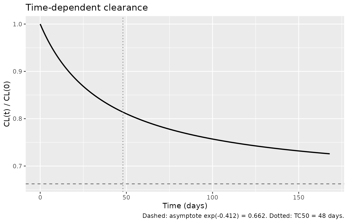
Time-dependent clearance of the typical AEGEAN patient over 24 weeks, with the asymptotic 33.8% reduction shown as a dashed line and TC50 = 48 days dotted.
Body weight on clearance and central volume (Results 3.2)
This is the load-bearing covariate check, and it is not circular. Results 3.2 reports two separate consequences of the same 95th-percentile body weight:
The impact of WT on CLss and V1 was also small, with a maximum change of +15.6% and +21.3% for the 95th percentile of WT, respectively.
The paper never prints what that 95th percentile is. So: back-solve
the weight from the V1 statement (which uses only
e_wt_vc), then use it to predict the CL
change (which uses only e_wt_cl) and compare against the
independently published +15.6%. A transcription error in either exponent
breaks the agreement.
# Back-solve WT95 from the published +21.3% on V1: (WT95/69.4)^0.503 = 1.213
wt95 <- 69.4 * 1.213^(1 / 0.503)
wt95
#> [1] 101.8781

# Predict the CL change at that same weight, from the model itself.
cl_change_pct <- 100 * (cl0(modifyList(ref_cov, list(WT = wt95))) / cl0(ref_cov) - 1)
#> ℹ omega/sigma items treated as zero: 'etalcl', 'etalvc', 'etacl_time_max'
#> ℹ omega/sigma items treated as zero: 'etalcl', 'etalvc', 'etacl_time_max'
cl_change_pct
#> [1] 15.61672

# Published +15.6%. One weight reproduces two independently published numbers.
stopifnot(abs(cl_change_pct - 15.6) < 0.5)

# And the back-solved weight must itself be a credible 95th percentile of a
# cohort with median 69.6 kg and range 31.0-175 kg (Table 1).
stopifnot(wt95 > 90, wt95 < 115)
The same arithmetic applied to albumin recovers the 5th percentile the paper used for its largest tornado bar (+21.3% on CLss):
alb05 <- 39 * 1.213^(-1 / 0.526)
alb05
#> [1] 27.01677

# Reproduces the published +21.3% on CLss, and must lie in the observed
# albumin range (Table 1: 3.70-78.0 g/L) below the 25th percentile of 35 g/L.
stopifnot(abs(100 * (cl0(modifyList(ref_cov, list(ALB = alb05))) / cl0(ref_cov) - 1) - 21.3) < 0.5)
#> ℹ omega/sigma items treated as zero: 'etalcl', 'etalvc', 'etacl_time_max'
#> ℹ omega/sigma items treated as zero: 'etalcl', 'etalvc', 'etacl_time_max'
stopifnot(alb05 > 3.7, alb05 < 35)
Mass balance
An exact identity that exercises the ODE system, the infusion and the
mg/L -> ug/mL scaling all at
once: at any time T, the drug eliminated so far equals the
amount dosed minus the amount still in the body, and the eliminated
amount is integral of cl(t) * Cc(t) dt. A fine grid on one
deterministic subject keeps the trapezoidal error small.
mb <- solve_one(aegean_typical, times = seq(0, 84, by = 0.005),
                dose_times = c(0, 21, 42, 63))
#> ℹ omega/sigma items treated as zero: 'etalcl', 'etalvc', 'etacl_time_max'

eliminated_integral <- sum(
  diff(mb$time) * (utils::head(mb$cl * mb$Cc, -1) + utils::tail(mb$cl * mb$Cc, -1)) / 2
)
in_body <- mb$central[nrow(mb)] + mb$peripheral1[nrow(mb)]
dosed <- 4 * 1500

c(dosed = dosed, in_body = in_body, eliminated = eliminated_integral,
  balance_pct = 100 * (eliminated_integral + in_body) / dosed - 100)
#>         dosed       in_body    eliminated   balance_pct
#>  6.000000e+03  1.271314e+03  4.728661e+03 -4.318354e-04

# Pure numerical (trapezoid) error -- both sides use the same drawn parameters,
# so a tight bound is correct here.
stopifnot(abs(100 * (eliminated_integral + in_body) / dosed - 100) < 0.5)
Body-weight quartile exposures recover the AEGEAN sex split
Supplementary Table S3 reports steady-state exposure as geometric means within body-weight quartiles, but gives no sex breakdown within those quartiles. That missing information turns into a strong, assumption-free test.
For a given weight, sex is the only other large covariate effect (16.6% on CL, 14.4% on Vc), so the all-male and all-female typical subjects bracket every achievable mixture. The published quartile value must fall inside that envelope – and where it falls inside implies a female fraction. Those implied fractions are a genuine prediction: they should decrease across weight quartiles (heavier patients are more often male) and should average to the AEGEAN female fraction of 35.1% from Table 2. Nothing in this calculation is tuned.
published_s3 <- tibble::tribble(
  ~wt_q, ~wt_pub, ~auclast, ~cmax, ~cmin,
  1L,     53.2,     8530,    777,   267,
  2L,     65.8,     7490,    673,   230,
  3L,     74.8,     6910,    613,   210,
  4L,     93.0,     6070,    539,   180
)

# Steady-state (4th Q3W interval, days 63-84) metrics for one typical subject.
ss_metrics <- function(wt, sexf) {
  cov <- modifyList(aegean_typical, list(WT = wt, SEXF = sexf))
  s <- solve_one(cov, times = sort(unique(c(seq(0, 84, by = 0.25), c(0, 21, 42, 63) + 1 / 24))),
                 dose_times = c(0, 21, 42, 63))
  ss <- s[s$time >= 63, ]
  c(
    auclast = sum(diff(ss$time) * (utils::head(ss$Cc, -1) + utils::tail(ss$Cc, -1)) / 2),
    cmax    = max(ss$Cc),
    cmin    = ss$Cc[ss$time == 84][1]
  )
}

envelope <- lapply(seq_len(nrow(published_s3)), function(k) {
  male   <- ss_metrics(published_s3$wt_pub[k], 0)
  female <- ss_metrics(published_s3$wt_pub[k], 1)
  pub    <- unlist(published_s3[k, c("auclast", "cmax", "cmin")])
  tibble::tibble(
    wt_q = published_s3$wt_q[k], metric = names(pub),
    Male = as.numeric(male), Published = as.numeric(pub), Female = as.numeric(female),
    # Where the published value sits in the male-to-female envelope, in log space.
    implied_female_frac = (log(pub) - log(male)) / (log(female) - log(male))
  )
}) |> bind_rows()
#> ℹ omega/sigma items treated as zero: 'etalcl', 'etalvc', 'etacl_time_max'
#> ℹ omega/sigma items treated as zero: 'etalcl', 'etalvc', 'etacl_time_max'
#> ℹ omega/sigma items treated as zero: 'etalcl', 'etalvc', 'etacl_time_max'
#> ℹ omega/sigma items treated as zero: 'etalcl', 'etalvc', 'etacl_time_max'
#> ℹ omega/sigma items treated as zero: 'etalcl', 'etalvc', 'etacl_time_max'
#> ℹ omega/sigma items treated as zero: 'etalcl', 'etalvc', 'etacl_time_max'
#> ℹ omega/sigma items treated as zero: 'etalcl', 'etalvc', 'etacl_time_max'
#> ℹ omega/sigma items treated as zero: 'etalcl', 'etalvc', 'etacl_time_max'

knitr::kable(
  envelope |>
    dplyr::rename(
      "Weight quartile" = wt_q, "Metric" = metric,
      "All male" = Male, "Published (Table S3)" = Published, "All female" = Female,
      "Implied female fraction" = implied_female_frac
    ),
  digits  = c(0, 0, 0, 0, 0, 3),
  caption = "Published Table S3 quartile exposures against the all-male / all-female typical-subject envelope. AUC in ug*day/mL, Cmax and Cmin in ug/mL."
)| Weight quartile | Metric | All male | Published (Table S3) | All female | Implied female fraction |
|---|---|---|---|---|---|
| 1 | auclast | 7476 | 8530 | 8793 | 0.813 |
| 1 | cmax | 700 | 777 | 825 | 0.636 |
| 1 | cmin | 225 | 267 | 274 | 0.870 |
| 2 | auclast | 6925 | 7490 | 8156 | 0.479 |
| 2 | cmax | 634 | 673 | 748 | 0.361 |
| 2 | cmin | 208 | 230 | 253 | 0.521 |
| 3 | auclast | 6610 | 6910 | 7791 | 0.270 |
| 3 | cmax | 597 | 613 | 705 | 0.155 |
| 3 | cmin | 198 | 210 | 241 | 0.305 |
| 4 | auclast | 6106 | 6070 | 7205 | -0.035 |
| 4 | cmax | 540 | 539 | 638 | -0.014 |
| 4 | cmin | 182 | 180 | 222 | -0.063 |
# 1. Every published value sits inside the envelope, give or take 3%. The
#    heaviest quartile is essentially all male, so it lands on (a hair below)
#    the male edge -- hence the small tolerance rather than a strict inequality.
tol <- 0.03
stopifnot(all(envelope$Published >= envelope$Male * (1 - tol)))
stopifnot(all(envelope$Published <= envelope$Female * (1 + tol)))

# 2. The implied female fraction falls monotonically with body weight, for all
#    three metrics independently. This is the prediction, not an input.
implied <- envelope |>
  tidyr::pivot_wider(id_cols = wt_q, names_from = metric, values_from = implied_female_frac) |>
  arrange(wt_q)
round(as.data.frame(implied), 3)
#>   wt_q auclast   cmax   cmin
#> 1    1   0.813  0.636  0.870
#> 2    2   0.479  0.361  0.521
#> 3    3   0.270  0.155  0.305
#> 4    4  -0.035 -0.014 -0.063

stopifnot(all(diff(implied$auclast) < 0))
stopifnot(all(diff(implied$cmax) < 0))
stopifnot(all(diff(implied$cmin) < 0))

# 3. Averaged over the four equally sized quartiles it reproduces the AEGEAN
#    female fraction of 35.1% (Table 2). A transcription error in e_wt_cl,
#    e_wt_vc, e_sexf_cl or e_sexf_vc breaks this.
mean_implied_female <- mean(envelope$implied_female_frac)
mean_implied_female
#> [1] 0.3581999

stopifnot(abs(mean_implied_female - 0.351) < 0.08)
Virtual AEGEAN cohort
The AEGEAN neoadjuvant regimen is durvalumab 1500 mg every 3 weeks
for four cycles with platinum-based chemotherapy
(CONMED_CHEMO = 1), given as a 1 h intravenous infusion.
Every published AEGEAN exposure metric (Tables S3 and S4) is derived
from this phase, with “steady state” defined in Methods 2.3 as
the fourth Q3W dose, i.e. the last dose before surgery
– so AUCss, Cmax,ss and Cmin,ss
are the fourth dosing interval, days 63 to 84.
Covariate distributions reproduce the AEGEAN column of Tables 1 and 2. Weight is drawn conditionally on sex, because Table S3 stratifies exposure by weight quartile and the sex mix genuinely differs across those quartiles; an independent draw would attribute the whole quartile spread to weight alone. See Assumptions and deviations.
set.seed(20260912)
n_sub <- 200L

sexf <- rbinom(n_sub, 1, 0.351)
cohort <- tibble::tibble(
  id       = seq_len(n_sub),
  SEXF     = sexf,
  # Sex-specific lognormal weight; the mixture reproduces the AEGEAN median of
  # 70.0 kg and mean 71.5 kg (SD 16.3) of Table 1.
  WT       = pmin(pmax(rlnorm(n_sub, log(ifelse(sexf == 1, 62.5, 74.0)), 0.20), 39), 152),
  ALB      = pmin(pmax(rnorm(n_sub, 40.7, 5.03), 20), 60),
  CRCL     = pmin(pmax(rlnorm(n_sub, log(84.0), 0.31), 30), 250),
  ECOG_GE1 = rbinom(n_sub, 1, 0.294),
  CONMED_CHEMO = 1,
  CONMED_TREMELIMUMAB = 0,
  regimen  = "AEGEAN neoadjuvant 1500 mg Q3W x4"
)

# Weight quartiles, matching the Table S3 stratification.
cohort$wt_q <- dplyr::ntile(cohort$WT, 4)

summary(cohort$WT)
#>    Min. 1st Qu.  Median    Mean 3rd Qu.    Max.
#>   39.00   58.35   68.43   69.45   79.57  118.14
knitr::kable(
  cohort |>
    group_by(`Weight quartile` = wt_q) |>
    summarise(
      N = n(),
      `WT geometric mean (kg)` = exp(mean(log(WT))),
      `Female (%)` = 100 * mean(SEXF),
      .groups = "drop"
    ),
  digits = 1,
  caption = "Simulated AEGEAN cohort by weight quartile. Compare the weight geometric means against Table S3: 53.2, 65.8, 74.8 and 93.0 kg."
)| Weight quartile | N | WT geometric mean (kg) | Female (%) |
|---|---|---|---|
| 1 | 50 | 51.0 | 66 |
| 2 | 50 | 63.6 | 38 |
| 3 | 50 | 73.1 | 28 |
| 4 | 50 | 89.3 | 14 |
dose_times <- c(0, 21, 42, 63)

# Observation grid: a regular backbone plus the exact end-of-infusion times
# (where Cmax falls) and the exact interval boundaries PKNCA needs.
obs_times <- sort(unique(c(
  seq(0, 84, by = 0.5),
  dose_times, dose_times + 1 / 24,
  63, 84
)))

ev <- rxode2::et(amt = 1500, time = dose_times, dur = 1 / 24, cmt = "central") |>
  rxode2::et(obs_times, cmt = "central") |>
  rxode2::et(id = seq_len(n_sub))

# Materialize to a data frame BEFORE attaching covariates: assigning a column
# onto an rxEt object is silently dropped by rxode2.
events <- as.data.frame(ev) |>
  left_join(select(cohort, -wt_q), by = "id")

stopifnot(!anyNA(events$WT), !anyNA(events$ALB), !anyNA(events$CRCL))
rxode2::rxSetSeed(20260912)
sim <- rxode2::rxSolve(mod, events = events, keep = "regimen") |>
  as.data.frame()
#> ℹ parameter labels from comments will be replaced by 'label()'

stopifnot(nrow(sim) > 0, all(is.finite(sim$Cc)))
sim_q <- sim |>
  group_by(time) |>
  summarise(
    med = stats::median(Cc), lo = stats::quantile(Cc, 0.05),
    hi = stats::quantile(Cc, 0.95), .groups = "drop"
  )

ggplot(sim_q, aes(time, med)) +
  geom_ribbon(aes(ymin = lo, ymax = hi), fill = "steelblue", alpha = 0.25) +
  geom_line(linewidth = 0.8) +
  geom_vline(xintercept = dose_times, linetype = "dotted", colour = "grey60") +
  labs(
    x = "Time (days)", y = "Durvalumab (ug/mL)",
    title = "AEGEAN neoadjuvant phase: 1500 mg Q3W x 4",
    caption = "Dotted lines = dose times. Days 63-84 is the interval the paper calls steady state."
  )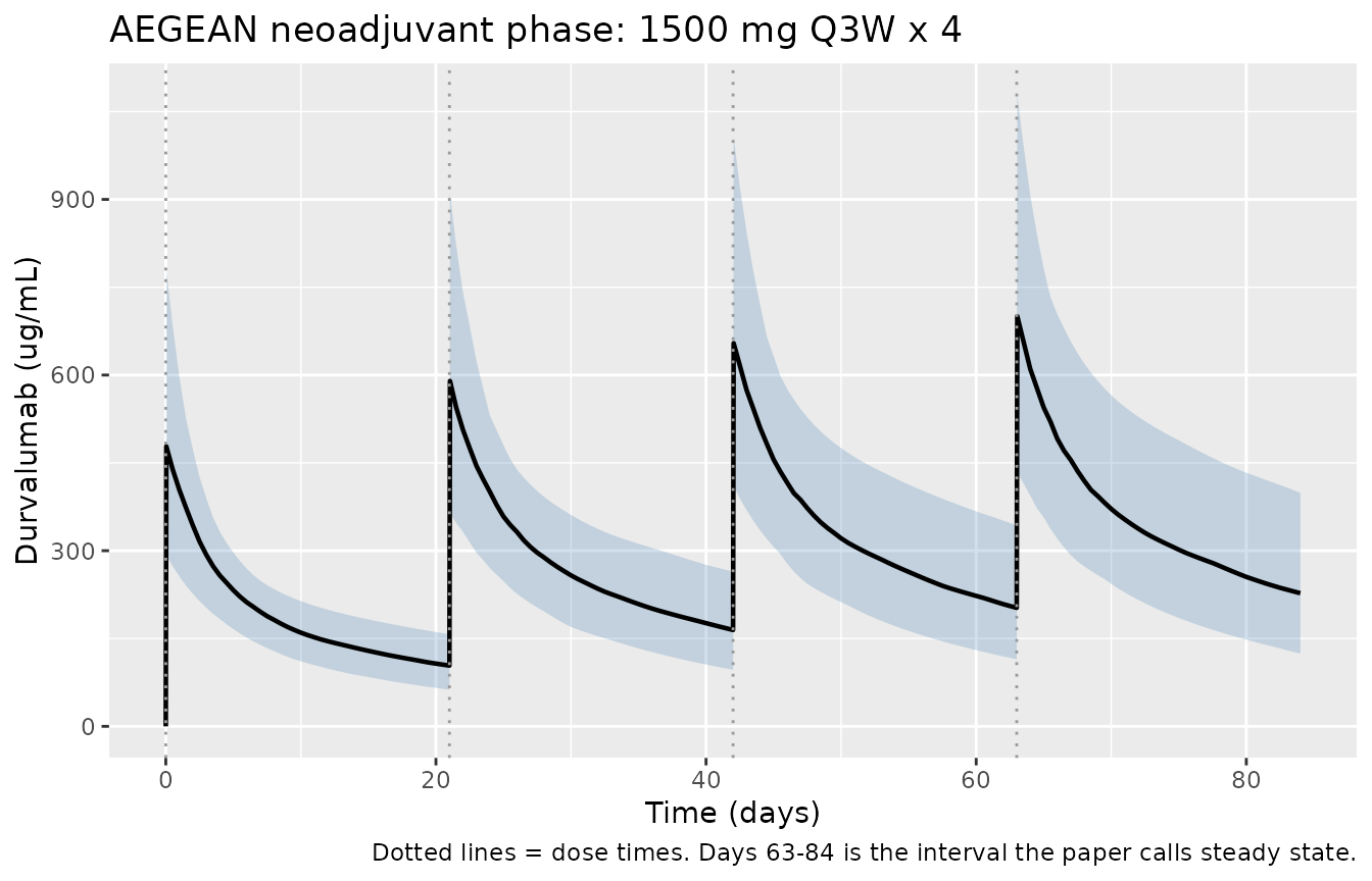
Simulated durvalumab serum concentrations over the four neoadjuvant Q3W cycles (n = 200). Solid line = median, ribbon = 5th-95th percentiles.
PKNCA validation
PKNCA::PKNCA.options(auc.method = "lin up/log down")

conc_df <- sim |>
  # Only !is.na(): a `time > 0` or `Cc > 0` filter would drop the rows PKNCA
  # needs to anchor each interval. The solve output has no evid column and
  # already contains only observation rows.
  filter(!is.na(Cc)) |>
  select(id, time, Cc, regimen)

# Both interval boundaries must actually be present for every subject.
stopifnot(all(tapply(conc_df$time, conc_df$id, function(x) 63 %in% x)))
stopifnot(all(tapply(conc_df$time, conc_df$id, max) == 84))

conc_obj <- PKNCA::PKNCAconc(conc_df, Cc ~ time | regimen + id)

dose_df <- events |>
  filter(evid == 1) |>
  select(id, time, amt, regimen)

dose_obj <- PKNCA::PKNCAdose(dose_df, amt ~ time | regimen + id)

# The fourth Q3W interval, days 63-84: the paper's definition of steady state.
#
# Note on Cmin,ss: PKNCA's `ctrough` returns NA here because day 84 carries no
# dose (in AEGEAN the fourth neoadjuvant dose is the last one before surgery),
# and its `cmin` would return the trough at the *start* of the interval -- which
# is lower than the one at the end, because drug is still accumulating at cycle
# 4. Cmin,ss is therefore read directly as the concentration at day 84, which is
# exactly the paper's definition, and asserted below to be the interval minimum
# after the peak.
intervals <- data.frame(
  start   = 63,
  end     = 84,
  cmax    = TRUE,
  tmax    = TRUE,
  auclast = TRUE
)

nca_res <- PKNCA::pk.nca(PKNCA::PKNCAdata(conc_obj, dose_obj, intervals = intervals))

cmin_ss <- sim |>
  filter(time == 84) |>
  select(id, cmin = Cc)

# It really is the post-peak minimum of the interval, for every subject.
post_peak_min <- sim |>
  filter(time > 63 + 1 / 24) |>
  group_by(id) |>
  summarise(m = min(Cc), .groups = "drop")
stopifnot(all(abs(post_peak_min$m - cmin_ss$cmin[match(post_peak_min$id, cmin_ss$id)]) < 1e-8))

nca_wide <- as.data.frame(nca_res) |>
  select(id, PPTESTCD, PPORRES) |>
  tidyr::pivot_wider(names_from = PPTESTCD, values_from = PPORRES) |>
  left_join(cmin_ss, by = "id") |>
  left_join(select(cohort, id, WT, SEXF, wt_q), by = "id")

stopifnot(nrow(nca_wide) == n_sub)
stopifnot(all(is.finite(nca_wide$cmax)), all(is.finite(nca_wide$auclast)),
          all(is.finite(nca_wide$cmin)))

knitr::kable(
  as.data.frame(nca_res) |>
    group_by(`NCA parameter` = PPTESTCD) |>
    summarise(
      Median = stats::median(PPORRES), P25 = stats::quantile(PPORRES, 0.25),
      P75 = stats::quantile(PPORRES, 0.75), .groups = "drop"
    ) |>
    dplyr::rename("25th pct" = P25, "75th pct" = P75),
  digits  = 1,
  caption = "Simulated steady-state NCA over the fourth Q3W interval (days 63-84), n = 200. cmax and ctrough in ug/mL, auclast in ug*day/mL, tmax in days."
)| NCA parameter | Median | 25th pct | 75th pct |
|---|---|---|---|
| auclast | 7198.9 | 5844.3 | 8513.8 |
| cmax | 665.6 | 553.6 | 780.3 |
| tmax | 0.0 | 0.0 | 0.0 |
Comparison against published NCA
Supplementary Table S4 reports the model-predicted steady-state exposure of all 385 AEGEAN PK-evaluable patients as geometric means, split into non-Chinese (n = 343) and Chinese (n = 42). The two differ by under 8%, so the simulated cohort is compared against the non-Chinese column, which carries 89% of the patients. The geometric mean is the right statistic here: for a log-normal distribution it is the typical value, which is what the model predicts.
geomean <- function(x) exp(mean(log(x)))

published_s4 <- tibble::tibble(
  regimen = "AEGEAN neoadjuvant 1500 mg Q3W x4",
  auclast = 7190, cmax = 645, cmin = 219
)

simulated_s4 <- nca_wide |>
  summarise(
    regimen = "AEGEAN neoadjuvant 1500 mg Q3W x4",
    auclast = geomean(auclast), cmax = geomean(cmax), cmin = geomean(cmin)
  )

cmp_s4 <- nlmixr2lib::ncaComparisonTable(
  simulated     = simulated_s4,
  reference     = published_s4,
  by            = "regimen",
  units         = c(auclast = "ug*day/mL", cmax = "ug/mL", cmin = "ug/mL"),
  tolerance_pct = 20
)

knitr::kable(
  cmp_s4,
  digits  = 1,
  caption = "Simulated vs. published (Table S4, non-Chinese column) steady-state exposure over the fourth Q3W interval. * differs from reference by >20%."
)| NCA parameter | regimen | Reference | Simulated | % diff |
|---|---|---|---|---|
| Cmax (ug/mL) | AEGEAN neoadjuvant 1500 mg Q3W x4 | 645 | 661 | +2.4% |
| Cmin (ug/mL) | AEGEAN neoadjuvant 1500 mg Q3W x4 | 219 | 213 | -2.6% |
| AUClast (ug*day/mL) | AEGEAN neoadjuvant 1500 mg Q3W x4 | 7190 | 7130 | -0.9% |
# `ncaComparisonTable()` renders its "% diff" column as TEXT, so recompute the
# difference numerically rather than parsing the rendered column.
pct_diff_s4 <- 100 * (
  unlist(simulated_s4[, c("auclast", "cmax", "cmin")]) /
    unlist(published_s4[, c("auclast", "cmax", "cmin")]) - 1
)
round(pct_diff_s4, 1)
#> auclast    cmax    cmin
#>    -0.9     2.4    -2.6

# Centre: a mis-transcribed clearance, volume, dose, exponent or unit moves the
# whole distribution by tens of percent. Raising CL from 0.285 to 0.385 L/day,
# for instance, drops steady-state AUC by about a quarter. Measured while
# authoring: -0.6% (AUC), +2.4% (Cmax) and -2.2% (Cmin) for this 200-subject
# draw. 10 leaves room for the cohort to be redrawn on a different rxode2
# build while still going red for a real transcription error.
stopifnot(max(abs(pct_diff_s4)) < 10)

# The simulated cohort must also reproduce the published weight ordering: both
# CL and Vc rise with body weight, so exposure falls across weight quartiles
# (Table S3: 8530 -> 7490 -> 6910 -> 6070 ug*day/mL).
by_quartile <- nca_wide |>
  group_by(wt_q) |>
  summarise(
    `WT geometric mean (kg)` = geomean(WT),
    `AUC (ug*day/mL)`        = geomean(auclast),
    `Cmax (ug/mL)`           = geomean(cmax),
    `Cmin (ug/mL)`           = geomean(cmin),
    .groups = "drop"
  ) |>
  arrange(wt_q)

knitr::kable(
  dplyr::rename(by_quartile, "Weight quartile" = wt_q),
  digits  = 1,
  caption = "Simulated steady-state exposure by weight quartile. Compare against Table S3 (53.2/65.8/74.8/93.0 kg; AUC 8530/7490/6910/6070), noting that the simulated quartile weights differ from the published ones -- the like-for-like comparison is the deterministic envelope check above."
)| Weight quartile | WT geometric mean (kg) | AUC (ug*day/mL) | Cmax (ug/mL) | Cmin (ug/mL) |
|---|---|---|---|---|
| 1 | 51.0 | 8438.8 | 807.8 | 257.8 |
| 2 | 63.6 | 7195.8 | 653.5 | 218.0 |
| 3 | 73.1 | 6752.0 | 619.0 | 200.5 |
| 4 | 89.3 | 6297.1 | 583.2 | 183.4 |
Assumptions and deviations
-
The exposure-response models are not packaged. Three ER layers are reported and none is reconstructable:
Event-free survival (Cox PH). Supplementary Table S5 lists all 26 stepwise candidates – including every exposure metric – and none met the
P < 0.01entry criterion (the smallest waslogBLTatP= 0.0318), so the final model is the covariate-free base model with-2LL= 996.7555. Its baseline hazard is never reported, so it cannot be simulated.-
pCR and safety (binary logistic regression). Tables S6-S9 report an exposure slope for each endpoint-by-metric pair but no intercept, and a logistic model cannot yield a probability without one. The mandatory figure-panel check was run: Figure 5 (pCR and grade >= 3 treatment-related AEs vs
AUC1dandAUCss) and Figure S2 (AESI and discontinuation) draw the fitted curves and their confidence bands, but print no coefficients in the panels. No intercept appears anywhere in the article or the supplement, so none could be recovered without digitising a curve for a relationship the authors themselves report as flat. The slopes are preserved here instead:Endpoint (n) Cmax,dose1Cmin,dose1AUCdose1Cmax,ssCmin,ssAUCsspCR (353), Table S6 -0.00203 -0.00178 -0.000156 -0.000654 +5.09e-05 -1.22e-05 Grade >= 3 TRAE (385), Table S7 -0.00183 -0.00534 -0.000202 -0.00112 -0.00188 -7.77e-05 Grade >= 3 AESI (385), Table S8 -0.00184 -0.0101 -0.000319 -0.00156 -0.00369 -0.000142 AE leading to discontinuation (385), Table S9 +0.000946 -0.000145 -4.44e-05 -0.000228 -0.000462 -9.78e-06 All 24 are non-significant (
P= 0.202-0.979 by likelihood ratio test), and every 95% confidence interval spans zero. This mirrors the sibling extractionAbegesah_2025_durvalumab.
IIV on the time-varying-CL asymptote is additive, not log-normal. Table 3 reports
ETA Tmax= 0.0534 but Zhao 2026 prints onlyexp(eta_i)on CL itself and never states the form forTmax. The model follows the idiom verified in the sibling AstraZeneca modelHwang_2022_tremelimumab– same modelling group, same senior author (Zhou D), sameEMPIR = Tmax * TIME^LAM / (TC50^LAM + TIME^LAM)parameterization – whose published NONMEM control stream definesTmax_i = THETA + ETA, and whichAbegesah_2025_durvalumabalso follows. A log-normal form is impossible here in any case becausecl_time_maxis negative. Note the 56.5% shrinkage on this eta: the published estimate is weakly informed by the data.Infusion duration is assumed to be 1 hour. Zhao 2026 does not state the AEGEAN infusion duration. One hour is the approved durvalumab administration and the value used by the sibling vignette
Abegesah_2025_durvalumab. The choice is nearly immaterial to AUC and trough, and movesCmaxby well under the 20% comparison tolerance, because the 1 h infusion is very short relative to the ~14-21 day half-life.Weight is simulated conditionally on sex. Table 1 reports the AEGEAN weight distribution and the sex split but not weight within sex. Sampling weight independently of sex would make the Table S3 weight quartiles sex-balanced, when in the real cohort the light quartiles are disproportionately female – and female sex carries a further 16.6% lower CL. The sex-specific medians used here (74.0 kg male, 62.5 kg female, both
sdlog= 0.20) are chosen to reproduce the published pooled median of 70.0 kg and mean of 71.5 kg; they are not published values. Albumin, creatinine clearance and ECOG are drawn independently, which remains a simplification of the real correlation structure. Note that no published comparison depends on this choice: the pooled Table S4 check is a whole-cohort geometric mean, and the Table S3 quartile check is done deterministically against the all-male/all-female envelope, which needs no assumption about the sex-weight relationship at all. The conditional draw only makes the simulated cohort’s own quartile table look like the published one.Cmin,ss is read as the concentration at day 84, not from PKNCA. PKNCA’s
ctroughreturnsNAfor this interval because day 84 carries no dose – the fourth neoadjuvant dose is the last before surgery – and itscminwould return the trough at the start of the interval, which is lower because drug is still accumulating at cycle 4. Day 84 is exactly the paper’s definition ofCmin,ss, and the vignette asserts it equals the post-peak interval minimum for every subject.CmaxandAUCstill come from PKNCA.cl_time_max,cl_t50andcl_time_hilltrigger aparameter_namingconvention warning asking for al-prefixed log-transformed name. The warning does not apply:cl_time_maxis negative (-0.412), solog()of it does not exist, andcl_time_hillisfixed(1.00). The already-merged siblingAbegesah_2025_durvalumabemits exactly the same three warnings for exactly the same parameters; this model is consistent with it.The
CRCLregister entry is BSA-normalized; this model’s is not. Table 1 reports “Creatinine clearance (mL/min)” with no BSA normalization, and the 85.66 normalizer printed inCL_cont.covis on that raw scale. The per-model unit is thereforemL/min, matching the sibling durvalumab modelsAbegesah_2025_durvalumab(85.66) anddeVries_2025_durvalumab(85.65).CONMED_CHEMOis time-varying in AEGEAN and is held at 1 here. The neoadjuvant phase iscomb = 1(durvalumab + platinum doublet) and the post-surgical adjuvant phase iscomb = 0(monotherapy). Every published AEGEAN exposure metric is derived from the neoadjuvant phase, so this vignette simulates only that phase and holdsCONMED_CHEMO = 1. A user simulating the full perioperative regimen must switch the column to 0 at surgery.No AEGEAN patient received tremelimumab, so
CONMED_TREMELIMUMABis 0 throughout. Thee_treme_clcoefficient is exercised only by the POSEIDON stratum of the pooled dataset.
Errata
Table 3 gives the wrong unit for
Tmax change CL. The Unit column reads “L/day” for that row. It is a unitless log-scale change: it enters the model asexp(Tmax * t / (TC50 + t)), a dimensionless multiplier on CL, and the Discussion interprets it as a percentage (“clearance could decrease by a maximum of 34%”, which is1 - exp(-0.412)= 33.8%). The neighbouringTC50row is correctly labelled “day”. The model treats it as unitless.Tables 1 and 2 summarise N = 3212, but the analysis dataset is N = 3205. Results 3.1 states both: 2827 + 385 = 3212 patients entered, 7 were excluded for physiologically impossible covariate values, and “12 466 PK samples from 3205 patients … were available in the final dataset for analysis”. The demographic percentages quoted in this vignette are the Table 1/2 values (denominator 3212);
population$n_subjectsrecords 3205.Table S1 understates the AEGEAN sample size. It lists “~200” subjects for AEGEAN, whereas the Results, Tables 1 and 2, and the ER analysis all use 385 PK-evaluable AEGEAN patients. The “~200” appears to be a planned-enrolment figure carried over from the analysis plan; 385 is used throughout this extraction.
The
Tmax change CLbootstrap interval is printed in descending order. Table 3 shows[-0.465; -0.360]for a bootstrap median of -0.414, i.e. lower bound first in magnitude but the interval reads high-to-low as printed. The same descending convention is used for every negative-valued row (albumin, ECOG, sex, COMB1, COMB2, sex on V1). No values are affected; it is a presentation artifact of negative numbers in that table.