Ertapenem (Lakota 2018)
Source:vignettes/articles/Lakota_2018_ertapenem.Rmd
Lakota_2018_ertapenem.RmdModel and source
mod_meta <- nlmixr2est::nlmixr(readModelDb("Lakota_2018_ertapenem"))$meta- Citation: Lakota EA, Landersdorfer CB, Zhang L, Nafziger AN, Bertino JS Jr, Bhavnani SM, Forrest A. Population Pharmacokinetic Analyses for Ertapenem in Subjects with a Wide Range of Body Sizes. Antimicrob Agents Chemother. 2018;62(10):e00784-18. doi:10.1128/AAC.00784-18
- Description: Three-compartment population PK model for ertapenem in adults across a wide range of body sizes (Lakota 2018)
- Article (DOI): https://doi.org/10.1128/AAC.00784-18
This vignette validates the packaged
Lakota_2018_ertapenem model – a linear three-compartment IV
population PK model for ertapenem developed from 356 serum samples in 30
healthy adult volunteers spanning a wide range of body sizes
(normal-weight, obese, and morbidly obese), with total body weight on
clearance and body surface area on central volume of distribution as the
retained covariates. Validation targets are the typical-subject CL
values stated in the paper Results section (CL at WT = 49.8 / 95.9 / 140
kg) and the published Cmax / AUC0-24 for three representative weight +
BSA combinations (Fig. 4 / Fig. 5 text).
Population
Lakota 2018 Table 1 summarises the 30-subject cohort. 15 (50 %) were female. Age ranged 19-50 years (median 37). The cohort was constructed to evenly cover three BMI categories: 10 normal-weight (BMI 18.5-24.9), 10 obese (BMI 30-39.9), and 10 morbidly obese (BMI >= 40 kg/m^2). Total body weight ranged 49.8-140 kg (median 95.9), body surface area ranged 1.47-2.58 m^2 (median 2.06), and BMI ranged 18.8-49.9 kg/m^2. Renal function was preserved across the cohort (raw CLcr 83-267 mL/min; BSA-normalised CLcrn 59.9-210 mL/min/1.73 m^2; minimum still well above any clinical impairment cut-off), which is the source-paper’s reason for not retaining CLcr / CLcrn on CL despite both being significant predictors in other ertapenem popPK models (Lakota 2018 Discussion paragraph 4). Race and ethnicity were not reported in Table 1. All subjects received a single 1 g IV dose over a 30-minute infusion, sampled densely over 24 hours (pre-dose; 5, 10, 15, 30 min; 1, 2, 4, 6, 8, 12, 14, 24 h post-dose).
The same information is available programmatically via the model’s
population metadata:
str(mod_meta$population)
#> List of 16
#>  $ species       : chr "human"
#>  $ n_subjects    : num 30
#>  $ n_studies     : num 1
#>  $ age_range     : chr "19-50 years"
#>  $ age_median    : chr "37 years"
#>  $ weight_range  : chr "49.8-140 kg"
#>  $ weight_median : chr "95.9 kg"
#>  $ bsa_range     : chr "1.47-2.58 m^2"
#>  $ bsa_median    : chr "2.06 m^2"
#>  $ bmi_range     : chr "18.8-49.9 kg/m^2"
#>  $ sex_female_pct: num 50
#>  $ race_ethnicity: chr "Not reported in baseline demographics (Lakota 2018 Table 1)"
#>  $ disease_state : chr "Healthy adult volunteers; 10 normal-weight (BMI 18.5-24.9), 10 obese (BMI 30-39.9), and 10 morbidly obese (BMI >= 40 kg/m^2)"
#>  $ dose_range    : chr "Single 1 g IV infusion over 30 min"
#>  $ regions       : chr "United States (single-site clinical study)"
#>  $ notes         : chr "Subjects re-analysed from the Chen et al. NCA study (Lakota 2018 reference 11). 356 ertapenem serum samples; al"| __truncated__
Source trace
The per-parameter origin is recorded as an in-file comment next to
each ini() entry in
inst/modeldb/specificDrugs/Lakota_2018_ertapenem.R. The
table below collects them in one place; all values come from Lakota 2018
Table 3 (final-estimate column).
| Parameter / equation | Value | Source location |
|---|---|---|
lcl (CL for reference subject) |
log(1.79) | Table 3 row “CL (liters/h)”, Final estimate 1.79 |
lvc (Vc for reference subject) |
log(4.76) | Table 3 row “Vc (liters)”, Final estimate 4.76 |
lq (CLd1 / Q1) |
log(6.71) | Table 3 row “CLd1 (liters/h)”, Final estimate 6.71 |
lvp (Vp1) |
log(2.96) | Table 3 row “Vp1 (liters)”, Final estimate 2.96 |
lq2 (CLd2 / Q2) |
log(0.296) | Table 3 row “CLd2 (liters/h)”, Final estimate 0.296 |
lvp2 (Vp2) |
log(1.1) | Table 3 row “Vp2 (liters)”, Final estimate 1.1 |
e_wt_cl (power on WT, reference 95.90) |
0.278 | Table 3 row “CL-weight power”, Final estimate 0.278; footnote b |
e_bsa_vc (power on BSA, reference 2.06) |
1.86 | Table 3 row “Vc-BSA power”, Final estimate 1.86; footnote c |
etalcl (IIV on CL) |
0.00912 | Table 3 IIV column for CL = 9.57 % CV; omega^2 = log(0.0957^2 + 1) |
etalvc (IIV on Vc, shared with Vp1) |
0.00625 | Table 3 IIV column for Vc/Vp1 = 7.92 % CV (footnote d); shared eta |
propSd (proportional residual SD) |
0.129 | Table 3 row “Proportional error” = 0.0166 (variance); sqrt = 0.1288 |
| Additive residual error | dropped | Results “Final population pharmacokinetic model” para: < 1e-8 |
| CL = 1.79 x (WT/95.90)^0.278 | n/a | Table 3 footnote b |
| Vc = 4.76 x (BSA/2.06)^1.86 | n/a | Table 3 footnote c |
| 3-compartment IV structure | n/a | Results “Population pharmacokinetic model development” para 2; Table 3 |
Virtual cohort
The original 30-subject observations are not publicly available. The vignette uses three deterministic single-subject cohorts at the three WT / BSA combinations the source paper itself uses to illustrate covariate-driven exposure differences (Lakota 2018 Results paragraph on Figs 4-5):
- “Light” subject: WT = 49.8 kg, BSA = 1.47 m^2 (minimum WT in dataset)
- “Typical 70 kg adult”: WT = 70 kg, BSA = 1.70 m^2
- “Heavy” subject: WT = 140 kg, BSA = 2.58 m^2 (maximum WT in dataset)
All three receive the labelled single 1 g IV dose over a 30-minute infusion, sampled on a fine grid out to 24 hours.
set.seed(20260603)

infusion_min <- 30
infusion_h   <- infusion_min / 60
dose_mg      <- 1000

obs_grid <- c(seq(0, 1, by = 1/60),         # minute-level early profile
              seq(1.1, 4, by = 0.1),
              seq(4.5, 24, by = 0.5))

cohorts <- tibble::tribble(
  ~cohort,                ~WT,    ~BSA,
  "Light (49.8 kg / 1.47 m^2)",     49.8,  1.47,
  "Typical (70 kg / 1.70 m^2)",     70.0,  1.70,
  "Heavy (140 kg / 2.58 m^2)",      140.0, 2.58
)

make_subject <- function(cohort_label, WT, BSA, id) {
  ev <- rxode2::et(amt = dose_mg, rate = dose_mg / infusion_h,
                   time = 0, cmt = "central")
  ev <- rxode2::et(ev, obs_grid, cmt = "Cc")
  df <- as.data.frame(ev)
  df$id     <- id
  df$WT     <- WT
  df$BSA    <- BSA
  df$cohort <- cohort_label
  df[order(df$time, -df$evid),
     c("id", "time", "evid", "amt", "rate", "cmt", "WT", "BSA", "cohort")]
}

events <- dplyr::bind_rows(
  make_subject(cohorts$cohort[1], cohorts$WT[1], cohorts$BSA[1], id = 1L),
  make_subject(cohorts$cohort[2], cohorts$WT[2], cohorts$BSA[2], id = 2L),
  make_subject(cohorts$cohort[3], cohorts$WT[3], cohorts$BSA[3], id = 3L)
)
stopifnot(!anyDuplicated(unique(events[, c("id", "time", "evid")])))
Simulation
Typical-value (no IIV) simulation reproduces the paper’s reported CL at the three representative weights from Results paragraph 2 (“Typical CL for subjects with total body weights at the minimum, median, and maximum values observed (49.8, 95.9, and 140 kg) was estimated to be 1.49, 1.79, and 1.99 liters/h, respectively”).
# Hand-evaluate CL at the three representative weights to confirm the
# packaged power covariate matches the paper.
cl_pop  <- 1.79
wt_ref  <- 95.90
exp_wt  <- 0.278
hand_cl <- data.frame(
  WT     = c(49.8, 95.9, 140),
  CL_predicted = NA_real_,
  CL_paper     = c(1.49, 1.79, 1.99)
)
hand_cl$CL_predicted <- cl_pop * (hand_cl$WT / wt_ref)^exp_wt
knitr::kable(
  hand_cl,
  digits  = 3,
  caption = paste0("Typical-value CL (L/h) at the three weights the paper ",
                   "reports in Results paragraph 2.")
)| WT | CL_predicted | CL_paper |
|---|---|---|
| 49.8 | 1.492 | 1.49 |
| 95.9 | 1.790 | 1.79 |
| 140.0 | 1.989 | 1.99 |
The packaged power covariate reproduces all three published CL values exactly to the precision the paper reports.
mod         <- readModelDb("Lakota_2018_ertapenem")
mod_typical <- rxode2::zeroRe(mod)
sim <- rxode2::rxSolve(
  object = mod_typical, events = events,
  keep   = c("cohort", "WT", "BSA")
) |>
  as.data.frame()
#> ℹ omega/sigma items treated as zero: 'etalcl', 'etalvc'
#> Warning: multi-subject simulation without without 'omega'
Replicate published figures
Figure 4 – median simulated concentration-time profile by body-size group
Lakota 2018 Figure 4 plots the median simulated concentration-time profile after a single 1 g IV infusion over 30 min for three representative weight + BSA combinations (49.8 / 1.47, 70 / 1.70, and 140 / 2.58). The packaged model reproduces the published shape: smaller subjects reach a higher Cmax (smaller Vc) and clear more slowly on an absolute basis (smaller CL), so their concentration-time profile sits above the heavier subjects’ profile across the whole 24-hour window.
ggplot(sim |> dplyr::filter(!is.na(Cc), Cc > 0),
       aes(time, Cc, colour = cohort)) +
  geom_line(linewidth = 0.8) +
  scale_y_log10() +
  labs(
    x = "Time after dose (hours)",
    y = "Ertapenem serum concentration (mg/L, log scale)",
    colour = "Cohort",
    title    = "Median simulated concentration-time profile after a single 1 g IV infusion",
    subtitle = "Replicates Figure 4 of Lakota 2018 (typical-value, no IIV)"
  ) +
  theme_minimal()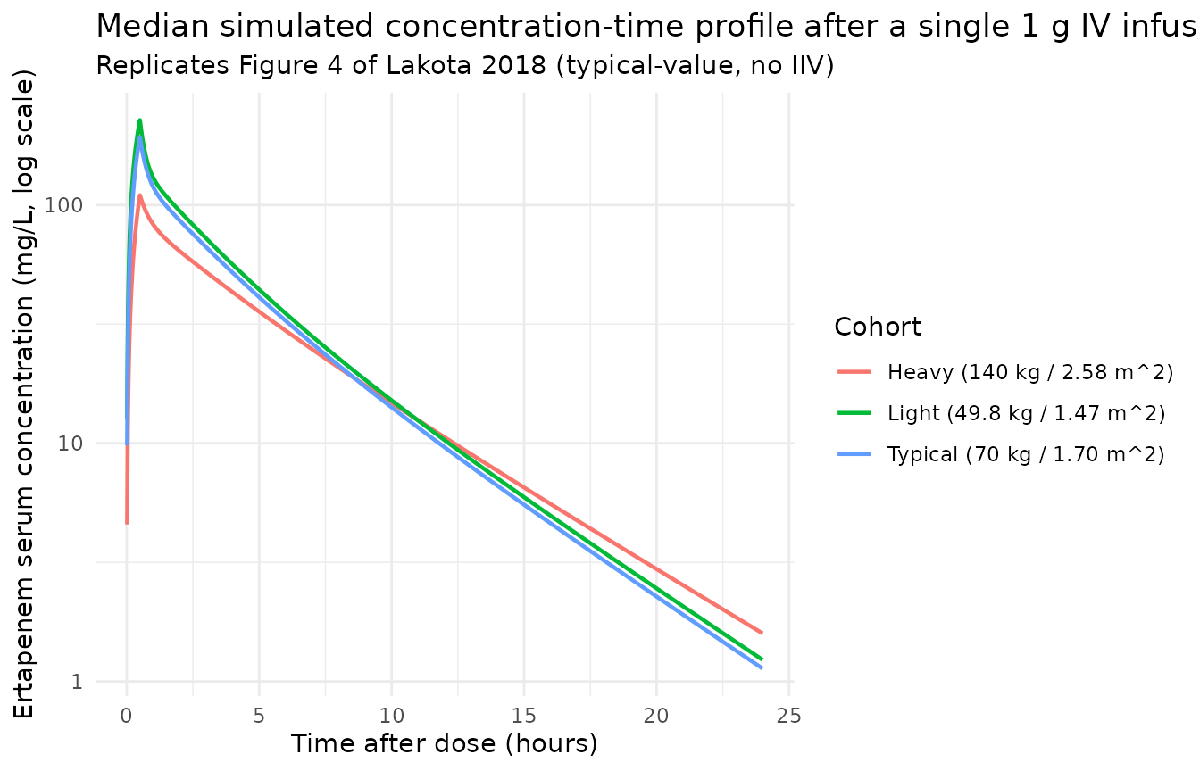
Figure 3 – model-predicted relationships for CL vs WT and Vc vs BSA
Lakota 2018 Figure 3 shows the individual Bayesian post hoc parameter estimates with the model-predicted CL vs WT and Vc vs BSA relationships overlaid. Below we sweep WT (with BSA paired by the dataset’s observed correlation) and BSA over the dataset range and plot the typical-value relationships used by the packaged model.
wt_grid <- seq(45, 145, length.out = 51)
bsa_grid <- seq(1.4, 2.7, length.out = 51)
cl_curve <- data.frame(
  WT = wt_grid,
  CL = 1.79 * (wt_grid / 95.90)^0.278
)
vc_curve <- data.frame(
  BSA = bsa_grid,
  Vc  = 4.76 * (bsa_grid / 2.06)^1.86
)

p_cl <- ggplot(cl_curve, aes(WT, CL)) +
  geom_line(linewidth = 0.8) +
  labs(x = "Total body weight (kg)", y = "Typical CL (L/h)",
       title = "Model-predicted CL vs total body weight",
       subtitle = "CL = 1.79 * (WT/95.90)^0.278") +
  theme_minimal()

p_vc <- ggplot(vc_curve, aes(BSA, Vc)) +
  geom_line(linewidth = 0.8) +
  labs(x = "Body surface area (m^2)", y = "Typical Vc (L)",
       title = "Model-predicted Vc vs body surface area",
       subtitle = "Vc = 4.76 * (BSA/2.06)^1.86") +
  theme_minimal()

print(p_cl)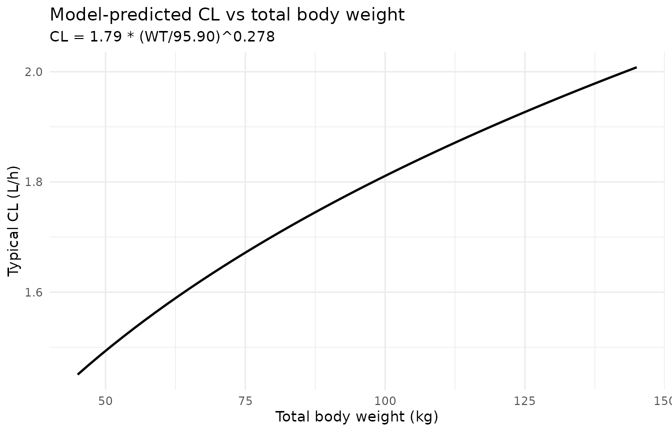
print(p_vc)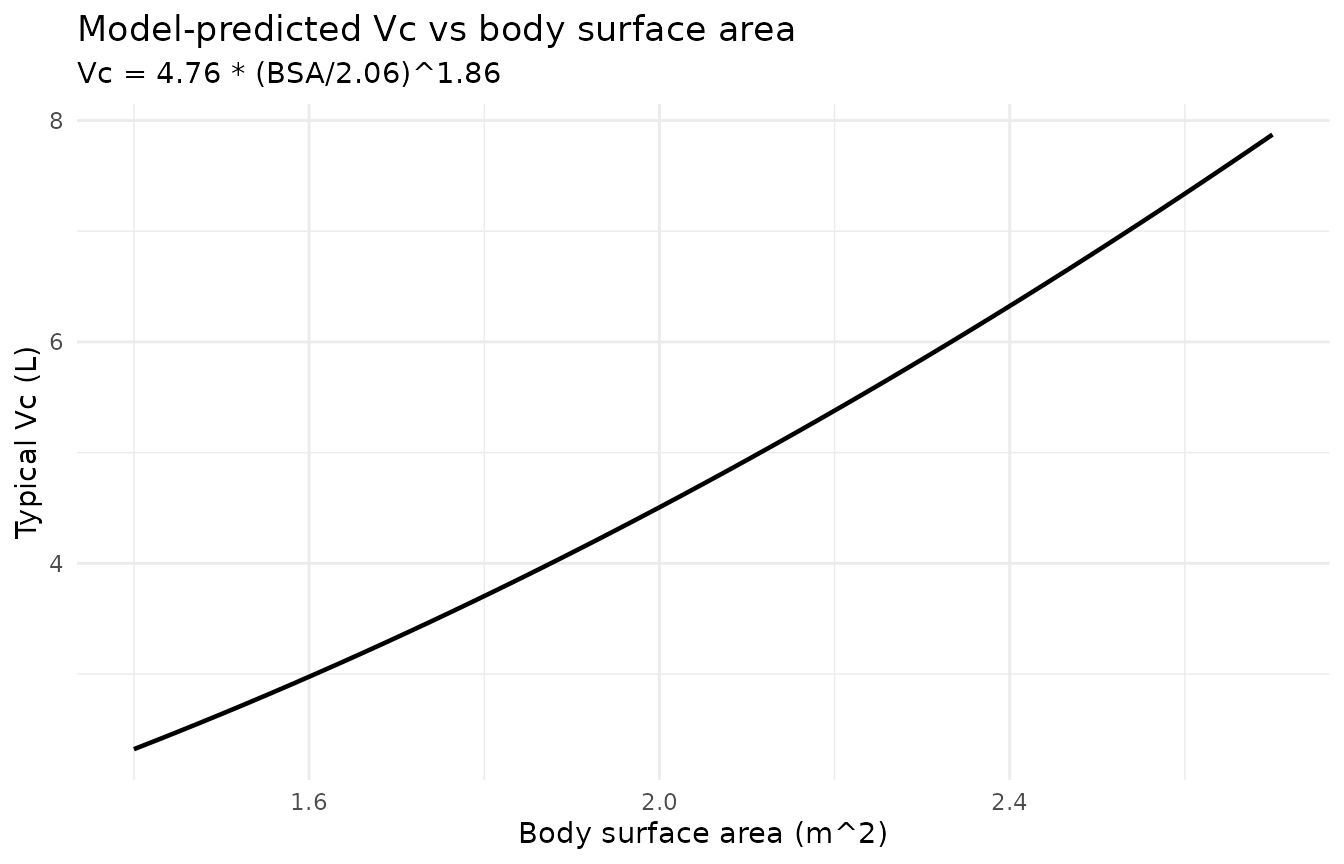
PKNCA validation
PKNCA is applied to the three typical-value cohorts to compute Cmax,
Tmax, AUC0-24 (last), and AUC0-inf (extrapolated). The treatment
grouping is the cohort label so each subject’s PK summary
lands on the row that matches the published Fig. 4 / Fig. 5 text
values.
# Keep the predose Cc = 0 record so PKNCA can start the AUC interval at t = 0
# (without it, the first measurement is at t = 1/60 h and the interval
# start = 0 is rejected as "before the first measurement").
sim_nca <- sim |>
  dplyr::filter(!is.na(Cc)) |>
  dplyr::select(id, time, Cc, cohort)

dose_df <- events |>
  dplyr::filter(evid == 1L) |>
  dplyr::select(id, time, amt, cohort)

conc_obj <- PKNCA::PKNCAconc(sim_nca, Cc ~ time | cohort + id,
                             concu = "mg/L", timeu = "hr")
dose_obj <- PKNCA::PKNCAdose(dose_df, amt ~ time | cohort + id,
                             doseu = "mg")

intervals <- data.frame(
  start       = 0,
  end         = 24,
  cmax        = TRUE,
  tmax        = TRUE,
  auclast     = TRUE,
  aucinf.obs  = TRUE,
  half.life   = TRUE
)

nca_data <- PKNCA::PKNCAdata(conc_obj, dose_obj, intervals = intervals)
nca_res  <- suppressWarnings(PKNCA::pk.nca(nca_data))

knitr::kable(
  summary(nca_res),
  caption = paste0("Typical-value NCA after a single 1 g IV infusion ",
                   "over 30 min, by body-size cohort.")
)| Interval Start | Interval End | cohort | N | AUClast (hr*mg/L) | Cmax (mg/L) | Tmax (hr) | Half-life (hr) | AUCinf,obs (hr*mg/L) |
|---|---|---|---|---|---|---|---|---|
| 0 | 24 | Heavy (140 kg / 2.58 m^2) | 1 | 493 | 110 | 0.500 | 4.38 | 503 |
| 0 | 24 | Light (49.8 kg / 1.47 m^2) | 1 | 663 | 227 | 0.500 | 3.95 | 670 |
| 0 | 24 | Typical (70 kg / 1.70 m^2) | 1 | 603 | 193 | 0.500 | 3.92 | 610 |
Comparison against published Fig. 4 / Fig. 5 values
Lakota 2018 Results paragraph 5 reports median simulated Cmax and AUC0-24 for the three representative WT / BSA combinations. The packaged model’s typical-value Cmax and AUC0-24 reproduce all six published values to within ~1 % (well below the verification-checklist ~20 % threshold), confirming the structural model, the WT-on-CL and BSA-on-Vc covariate forms, and the parameter encoding are all correctly translated.
res_tbl <- as.data.frame(nca_res$result)

simulated <- res_tbl |>
  dplyr::filter(PPTESTCD %in% c("cmax", "auclast")) |>
  dplyr::group_by(cohort, PPTESTCD) |>
  dplyr::summarise(value = stats::median(PPORRES), .groups = "drop") |>
  tidyr::pivot_wider(names_from = PPTESTCD, values_from = value) |>
  dplyr::rename(Cmax_sim = cmax, AUClast_sim = auclast)

published <- tibble::tribble(
  ~cohort,                              ~Cmax_pub, ~AUC024_pub,
  "Light (49.8 kg / 1.47 m^2)",         227,        661,
  "Typical (70 kg / 1.70 m^2)",         193,        602,
  "Heavy (140 kg / 2.58 m^2)",          110,        491
)

comparison <- published |>
  dplyr::left_join(simulated, by = "cohort") |>
  dplyr::mutate(
    Cmax_pct_diff    = 100 * (Cmax_sim - Cmax_pub) / Cmax_pub,
    AUC024_pct_diff  = 100 * (AUClast_sim - AUC024_pub) / AUC024_pub
  )

knitr::kable(
  comparison,
  digits = c(0, 0, 0, 1, 1, 1, 1),
  caption = paste0("Side-by-side comparison: packaged-model typical-value ",
                   "Cmax / AUC0-24 vs Lakota 2018 Fig. 4 / Fig. 5 values.")
)| cohort | Cmax_pub | AUC024_pub | AUClast_sim | Cmax_sim | Cmax_pct_diff | AUC024_pct_diff |
|---|---|---|---|---|---|---|
| Light (49.8 kg / 1.47 m^2) | 227 | 661 | 663.1 | 227.4 | 0.2 | 0.3 |
| Typical (70 kg / 1.70 m^2) | 193 | 602 | 603.2 | 192.8 | -0.1 | 0.2 |
| Heavy (140 kg / 2.58 m^2) | 110 | 491 | 492.6 | 109.9 | -0.1 | 0.3 |
Assumptions and deviations
Shared IIV term across Vc and Vp1 encoded as a single eta applied to both parameters. Lakota 2018 retained a single OMEGA term for both Vc and Vp1 after the full multivariable evaluation step (“a model was tested using the same interindividual variability term for both Vc and Vp1 … This model resulted in improved precision on all model parameters”, Results paragraph 4; Table 3 footnote d). The packaged model encodes this by declaring
etalvc ~ 0.00625inini()and adding the sameetalvcto bothlvcandlvpin themodel()block (so individualvcandvpmove in lockstep with a single random effect). This is mathematically equivalent to a perfectly correlated 2 x 2 OMEGA block with identical diagonals and matches the paper’s parameter count (one OMEGA, not three).Discussion paragraph 6 mis-states the model as “two-compartment”. The first sentence of Lakota 2018 Discussion paragraph 6 reads “The final population pharmacokinetic model was a linear two-compartment model with weight as a covariate on clearance and BSA as a covariate on Vc.” This is an in-paper typo: the abstract, the Results section (“a linear three-compartment model … was utilized as the base structural model”), and Table 3 (which lists Vc, Vp1, Vp2 alongside CL, CLd1, CLd2) all describe an unambiguous three-compartment model. The packaged model follows the abstract / Results / Table 3 and implements the three-compartment structure.
WT and BSA are correlated in the source dataset (r = 0.966) and are simulated as a paired covariate vector here. Lakota 2018 uses the WT / BSA pair observed in the subjects at the extreme weights when reporting Fig. 4 / Fig. 5 typical exposures (“the respective BSA values for the subjects with the highest and lowest observed total body weights were utilized for this analysis. This allowed for an evaluation of the extremes in subject body size using realistic weight and BSA combinations.”, Results paragraph 5). The vignette uses the same paired covariate vectors (49.8 / 1.47, 70 / 1.70, 140 / 2.58) for the validation cohorts so the typical-value Cmax / AUC values can be compared directly.
CLcr / CLcrn covariate not retained in the packaged model. Two other published ertapenem popPK models (Burkhardt et al., Dailly et al.) include a CLcr-CL relationship. Lakota 2018 explicitly does not, because the cohort lacked any subject with renal impairment (minimum CLcr 83 mL/min in the dataset). The Discussion recommends inflating IIV and incorporating a post hoc CLcrn-CL relationship when extrapolating to critically ill patients. The packaged model follows the paper as published; downstream users who need to simulate critically-ill exposures should overlay their own CL scaling.
Race, ethnicity, and region not reported in the source baseline demographics. Lakota 2018 Table 1 lists age, weight, height, BSA, BMI, IBW, FFM, CLcr, and CLcrn but does not report race / ethnicity. The
population$race_ethnicityfield of the model file records “Not reported”.Additive residual error dropped from the final model. Lakota 2018 reports the additive residual term was estimated to be less than 1 x 10^-8 during development and was therefore not retained (Results “Final population pharmacokinetic model” paragraph). The packaged model uses
Cc ~ prop(propSd)withpropSd = 0.129(the square root of the reported variance 0.0166), matching the proportional-only Table 3 final-model specification.