Tigecycline (Luo 2023) • nlmixr2lib

Model and source

ui <- rxode2::rxode(readModelDb("Luo_2023_tigecycline"))
#> ℹ parameter labels from comments will be replaced by 'label()'

Citation: Luo X, Wang S, Li D, Wen J, Sun N, Fan G. Population pharmacokinetics of tigecycline in critically ill patients. Front Pharmacol. 2023;14:1083464. doi:10.3389/fphar.2023.1083464
Description: One-compartment linear IV population PK model for tigecycline in critically ill adult ICU patients. Clearance decreases linearly with APACHE II score above the cohort median of 22.5 points, and central volume decreases linearly with age above the cohort median of 72 years. Fitted by NONMEM 7.3.0 FOCE-I to 143 steady-state plasma concentrations from 54 ICU patients on the licensed 100 mg loading / 50 mg q12h maintenance regimen.
Article: https://doi.org/10.3389/fphar.2023.1083464

Luo and colleagues fitted a one-compartment linear model with first-order elimination to 143 steady-state tigecycline plasma concentrations from 54 critically ill adults in a single Chinese ICU. Clearance falls with the APACHE II score and central volume falls with age; no other covariate survived the forward inclusion / backward elimination screen. The fitted model was then used in a Monte Carlo simulation to compute the probability of target attainment (PTA) and the cumulative fraction of response (CFR) for three dosing regimens against three infection-specific AUC0-24/MIC targets.

Population

pop <- ui$population

54 critically ill adults (44.4% female) treated at the Second Affiliated Hospital of Dalian Medical University between December 2017 and July 2018 contributed 143 plasma concentrations. The cohort was elderly (median age 72.0 years, IQR 57.5-80.3 years) and severely ill (median APACHE II 22.50, IQR 16.50-27.00). Median weight was 68.0 kg. All patients received the licensed regimen – a 100 mg IV loading dose followed by 50 mg q12h – for at least three days, and samples were drawn at steady state pre-dose and 1, 2 and 4 h after administration. Baseline demographics are Luo 2023 Table 1; the median observed concentration was 444.0 ng/mL (IQR 222.3-716.6).

The same information is available programmatically via readModelDb("Luo_2023_tigecycline")()$population.

Source trace

The per-parameter origin is recorded as an in-file comment next to each ini() entry in inst/modeldb/specificDrugs/Luo_2023_tigecycline.R. The table below collects them in one place for review.

Equation / parameter	Value	Source location
One-compartment linear model, first-order elimination	n/a	Results 3.2, first sentence; Abstract
`d/dt(central) <- -kel * central`	n/a	Results 3.2 (structural model)
`lcl` (CL at APACHE_II = 22.5)	`log(11.30)` L/h	Table 2 Theta1 = 11.30; Results eq. 1
`lvc` (Vc at AGE = 72)	`log(105.00)` L	Table 2 Theta2 = 105.00; Results eq. 2
`e_apache_cl` (slope of APACHE II on CL)	0.14 L/h per point	Table 2 Theta3 = 0.14; coefficient in Results eq. 1
`e_age_vc` (fractional slope of age on Vc)	0.0059 per year	Table 2 Theta4 = 0.0059; coefficient in Results eq. 2
`etalcl` (IIV on CL)	0.065 (variance)	Table 2 Omega1 = 0.065; exponential IIV per Results 3.2
`etalvc` (IIV on Vc)	0.160 (variance)	Table 2 Omega2 = 0.160; exponential IIV per Results 3.2
`expSd` (residual SD, log scale)	`sqrt(0.0316)` = 0.17776	Table 2 Sigma1 = 0.0316; exponential residual per Results 3.2
Centring of both covariate effects	22.5 points / 72 years	Table 1 cohort medians; see “Assumptions and deviations”
AUC0-24 = dose over 24 h / CL	n/a	Methods 2.6, last sentence
PK/PD targets 4.5 (HAP), 6.96 (cIAI), 17.9 (cSSSI)	n/a	Methods 2.6; Introduction
MIC distributions for the three pathogens	n/a	Table 3
Published PTA grid	n/a	Table 4

Virtual cohort

Original observed data are not publicly available. The cohort below draws APACHE II and age to match the medians and interquartile ranges of Luo 2023 Table 1 (normal approximations, truncated to the clinically admissible ranges: APACHE II is an integer 0-71 by construction, and the study enrolled adults only).

# set.seed() seeds R's RNG, not rxode2's simulation RNG, and rxode2's streams
# are partitioned per solver thread -- so the cohort below differs between a
# 2-core CI runner and a 16-thread workstation. Every assertion in this
# vignette is written so that it holds for any cohort the model can produce.
set.seed(20230313)

n_arm  <- 200L   # participants per regimen (skill cap)
tau    <- 12     # dosing interval (h)
t_inf  <- 0.5    # IV infusion duration (h); see "Assumptions and deviations"
n_dose <- 16L    # loading dose + 15 maintenance doses -> last dose at 180 h
ss_t0  <- 168    # start of the steady-state observation window (h)

# Table 1 reports medians and IQRs; convert IQR to an SD assuming normality.
apache_sd <- (27.00 - 16.50) / 1.349
age_sd    <- (80.3 - 57.5) / 1.349

regimens <- tibble::tribble(
  ~regimen,            ~load_mg, ~maint_mg,
  "100/50 mg q12h",     100,       50,
  "100/75 mg q12h",     100,       75,
  "200/100 mg q12h",    200,      100
)

obs_times <- seq(ss_t0, ss_t0 + 2 * tau, by = 0.25)

make_arm <- function(n, load_mg, maint_mg, label, id_offset = 0L) {
  subj <- tibble::tibble(
    id        = id_offset + seq_len(n),
    APACHE_II = round(pmin(71, pmax(0, rnorm(n, 22.50, apache_sd)))),
    AGE       = pmin(95, pmax(18, rnorm(n, 72.0, age_sd))),
    regimen   = label
  )
  doses <- subj |>
    tidyr::crossing(time = seq(0, by = tau, length.out = n_dose)) |>
    dplyr::mutate(
      evid = 1L,
      amt  = ifelse(time == 0, load_mg, maint_mg),
      rate = amt / t_inf,
      # cmt is the ODE STATE name, never the algebraic observable `Cc`.
      cmt  = "central"
    )
  obs <- subj |>
    tidyr::crossing(time = obs_times) |>
    dplyr::mutate(evid = 0L, amt = 0, rate = 0, cmt = "central")
  dplyr::bind_rows(doses, obs) |>
    dplyr::arrange(id, time, dplyr::desc(evid))
}

arms <- lapply(seq_len(nrow(regimens)), function(i) {
  make_arm(
    n         = n_arm,
    load_mg   = regimens$load_mg[i],
    maint_mg  = regimens$maint_mg[i],
    label     = regimens$regimen[i],
    id_offset = (i - 1L) * n_arm
  )
})
events <- dplyr::bind_rows(arms)

# Disjoint IDs across arms: duplicate IDs silently merge into one subject that
# receives the summed dose.
stopifnot(
  !anyDuplicated(unique(events[, c("id", "time", "evid")])),
  dplyr::n_distinct(events$id) == n_arm * nrow(regimens)
)

Simulation

mod <- readModelDb("Luo_2023_tigecycline")
sim <- rxode2::rxSolve(mod, events = events,
                       keep = c("regimen", "APACHE_II", "AGE")) |>
  as.data.frame()
#> ℹ parameter labels from comments will be replaced by 'label()'

# The solve must have produced the algebraic observable and the individual
# parameters the PTA section reads back out.
stopifnot(all(c("Cc", "cl", "vc") %in% names(sim)),
          sum(!is.na(sim$Cc)) > 0L,
          all(sim$Cc[!is.na(sim$Cc)] >= 0))

Steady-state concentration-time profiles

sim |>
  dplyr::filter(!is.na(Cc), time >= ss_t0) |>
  dplyr::mutate(tad = time - ss_t0) |>
  dplyr::group_by(regimen, tad) |>
  dplyr::summarise(
    Q05 = quantile(Cc, 0.05),
    Q50 = quantile(Cc, 0.50),
    Q95 = quantile(Cc, 0.95),
    .groups = "drop"
  ) |>
  ggplot(aes(tad, Q50, colour = regimen, fill = regimen)) +
  geom_ribbon(aes(ymin = Q05, ymax = Q95), alpha = 0.2, colour = NA) +
  geom_line() +
  labs(x = "Time after the start of the steady-state window (h)",
       y = "Tigecycline concentration (mg/L)",
       colour = NULL, fill = NULL,
       title = "Simulated steady-state tigecycline profiles",
       caption = paste("Median and 5th-95th percentile band,",
                       n_arm, "subjects per regimen."))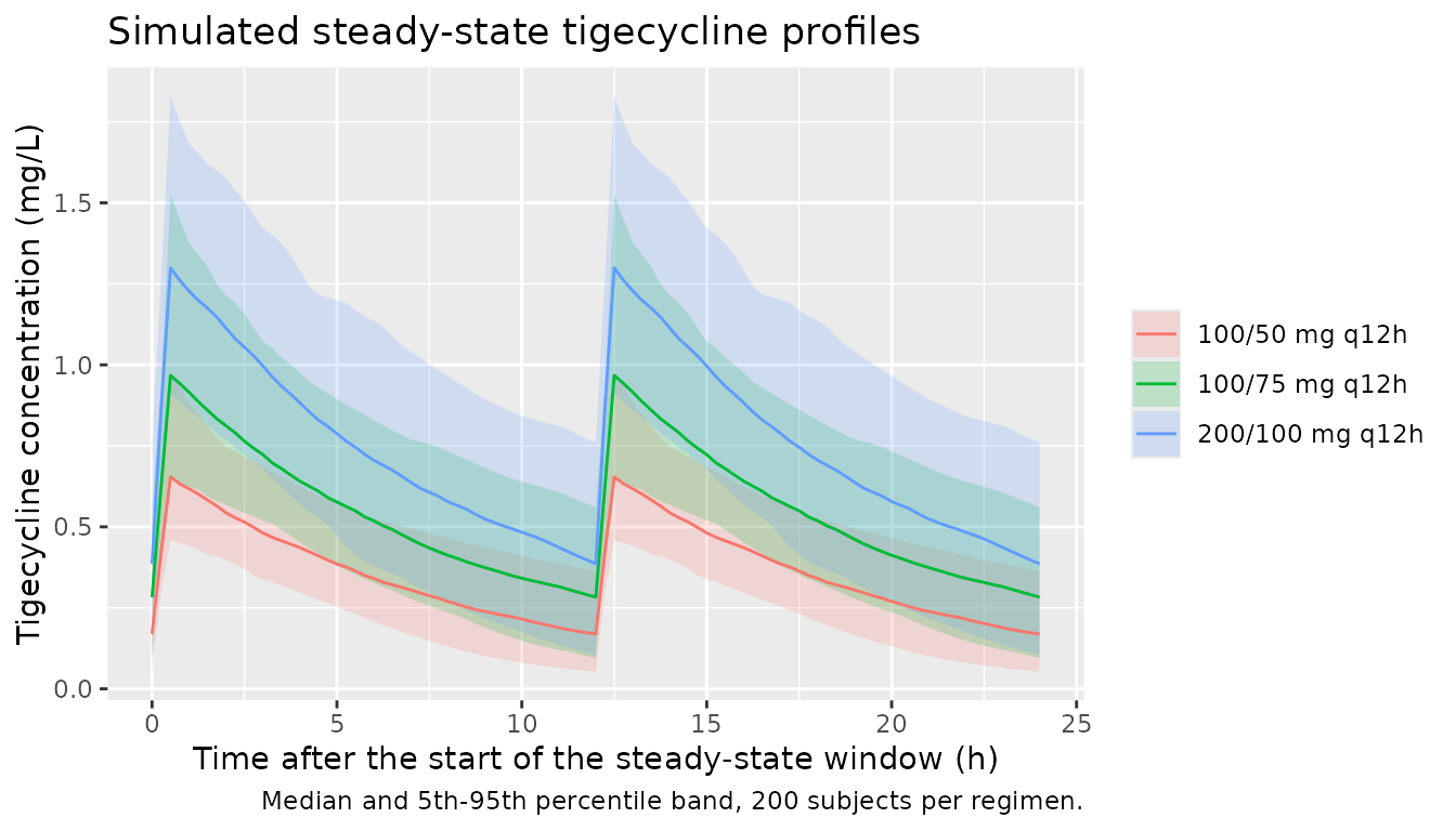

Does the covariate model reproduce the study’s own observed concentrations?

Luo 2023 prints the two parameter equations without a centring term (Results 3.2):

CL (L/h) = (11.30 - 0.14 x APACHE II score) x e^0.065        (eq. 1)
V  (L)   = [105.00 x (1 - 0.0059 x AGE)]   x e^0.160         (eq. 2)

Read literally, the typical patient (APACHE II 22.5, age 72) has CL = 8.15 L/h and V = 60.4 L. The packaged model instead centres both covariates at the cohort median, giving CL = 11.30 L/h and V = 105 L for that same patient – the values the paper itself calls the “population-typical values of CL and Vd”.

The check below decides between the two readings against the paper’s own reported data: the median observed concentration of 444.0 ng/mL over the study’s sampling design (steady state on 50 mg q12h; pre-dose, then 1, 2 and 4 h after the start of the infusion).

The uncentred reading is evaluated using the same packaged model, without re-implementing its arithmetic: because both effects are linear, evaluating the centred model at APACHE_II + 22.5 and AGE + 72 gives exactly the value the uncentred equations give at APACHE_II and AGE. The shifted ages are deliberately non-physiological; they are an algebraic device, not a cohort.

set.seed(4104)

sample_times <- ss_t0 + tau + c(-0.01, 1, 2, 4)   # pre-dose, then 1, 2, 4 h

chk_subj <- tibble::tibble(
  id        = seq_len(n_arm),
  APACHE_II = round(pmin(71, pmax(0, rnorm(n_arm, 22.50, apache_sd)))),
  AGE       = pmin(95, pmax(18, rnorm(n_arm, 72.0, age_sd)))
)

build_check_events <- function(subj) {
  doses <- subj |>
    tidyr::crossing(time = seq(0, by = tau, length.out = n_dose)) |>
    dplyr::mutate(evid = 1L, amt = ifelse(time == 0, 100, 50),
                  rate = amt / t_inf, cmt = "central")
  obs <- subj |>
    tidyr::crossing(time = sample_times) |>
    dplyr::mutate(evid = 0L, amt = 0, rate = 0, cmt = "central")
  dplyr::bind_rows(doses, obs) |>
    dplyr::arrange(id, time, dplyr::desc(evid))
}

# The exponential ("index") residual model is median-unbiased, so it cannot
# move the statistic being compared; it is applied anyway so the simulated
# spread is comparable to the observed IQR. The SD is read from the packaged
# model rather than retyped.
exp_sd <- ui$iniDf$est[ui$iniDf$name == "expSd"]
stopifnot(length(exp_sd) == 1L, is.finite(exp_sd))

median_conc <- function(subj) {
  s <- rxode2::rxSolve(mod, events = build_check_events(subj)) |>
    as.data.frame() |>
    dplyr::filter(!is.na(Cc), time %in% sample_times)
  stopifnot(nrow(s) == n_arm * length(sample_times))
  obs <- s$Cc * exp(rnorm(nrow(s), 0, exp_sd))
  c(q25 = unname(quantile(obs, 0.25)),
    med = unname(quantile(obs, 0.50)),
    q75 = unname(quantile(obs, 0.75)))
}

shifted <- chk_subj |>
  dplyr::mutate(APACHE_II = APACHE_II + 22.5, AGE = AGE + 72)

obs_med_mgL <- 444.0 / 1000   # Luo 2023 Table 1, converted from ng/mL

centring <- tibble::tibble(
  Reading = c("Centred (packaged model)", "Uncentred (eqs. 1-2 read literally)"),
  dplyr::bind_rows(median_conc(chk_subj), median_conc(shifted))
) |>
  dplyr::mutate(`Bias vs observed median (%)` = 100 * (med / obs_med_mgL - 1))

centring |>
  dplyr::rename(
    "Q1 (mg/L)"     = q25,
    "Median (mg/L)" = med,
    "Q3 (mg/L)"     = q75
  ) |>
  knitr::kable(
    digits  = c(0, 3, 3, 3, 1),
    caption = paste0(
      "Simulated steady-state concentrations on 50 mg q12h under the study's ",
      "own sampling design, against the observed median of 444.0 ng/mL ",
      "(IQR 222.3-716.6) reported in Luo 2023 Table 1."
    )
  )

Simulated steady-state concentrations on 50 mg q12h under the study’s own sampling design, against the observed median of 444.0 ng/mL (IQR 222.3-716.6) reported in Luo 2023 Table 1.
Reading	Q1 (mg/L)	Median (mg/L)	Q3 (mg/L)	Bias vs observed median (%)
Centred (packaged model)	0.307	0.460	0.604	3.6
Uncentred (eqs. 1-2 read literally)	0.419	0.694	0.935	56.3

bias <- centring$`Bias vs observed median (%)`
names(bias) <- c("centred", "uncentred")

# Cohort-derived quantities, so these are magnitude bounds with headroom rather
# than values taken from one run. Measured at both 2 and 16 rxode2 solver
# threads: +3.6% for the centred reading and +56.3% for the uncentred one. A
# mis-transcribed clearance, volume, dose or unit moves the centred figure by
# tens of percent and still breaks the first bound; the second bound still
# breaks if the two readings ever converge.
stopifnot(
  abs(bias[["centred"]]) < 25,
  bias[["uncentred"]] > 35
)

A converged FOCE-I fit whose reported goodness-of-fit is symmetric about the line of identity (Luo 2023 Figure 1) cannot overpredict the median of its own data by half. Two further internal checks point the same way and are reproduced below: the AUC0-24 column of Table 4, and the Monte Carlo PTA grid.

Table 4: AUC0-24 and the probability of target attainment

Methods 2.6 defines AUC0-24 as the 24 h dose divided by the individual’s clearance. The three AUC0-24 values printed in Table 4 therefore pin the typical clearance the authors simulated with.

auc_published <- c(`100/50 mg q12h` = 8.85,
                   `100/75 mg q12h` = 13.27,
                   `200/100 mg q12h` = 17.70)
dose24 <- c(`100/50 mg q12h` = 100, `100/75 mg q12h` = 150,
            `200/100 mg q12h` = 200)

implied_cl <- dose24 / auc_published

tibble::tibble(
  Regimen                  = names(auc_published),
  `Dose over 24 h (mg)`    = as.numeric(dose24),
  `AUC0-24 (mg*h/L)`       = as.numeric(auc_published),
  `Implied typical CL (L/h)` = as.numeric(implied_cl)
) |>
  knitr::kable(digits = 3,
               caption = "Luo 2023 Table 4: dose / AUC0-24 recovers the typical clearance.")

Luo 2023 Table 4: dose / AUC0-24 recovers the typical clearance.
Regimen	Dose over 24 h (mg)	AUC0-24 (mg*h/L)	Implied typical CL (L/h)
100/50 mg q12h	100	8.85	11.299
100/75 mg q12h	150	13.27	11.304
200/100 mg q12h	200	17.70	11.299


# Deterministic arithmetic on published numbers, so a tight bound is correct.
stopifnot(max(abs(implied_cl - 11.30)) < 0.01)

All three rows recover 11.30 L/h, which is the packaged model’s typical clearance at the median APACHE II of 22.5 – not the 8.15 L/h that eq. 1 gives there when read uncentred.

The converse check runs the packaged model forwards. With the random effects zeroed and the covariates set to the cohort medians, the steady-state AUC0-24 integrated from the solved profile must land on the published column.

mod_typ <- rxode2::zeroRe(mod)
#> ℹ parameter labels from comments will be replaced by 'label()'

typical_auc <- function(load_mg, maint_mg) {
  ev <- dplyr::bind_rows(
    tibble::tibble(id = 1L, time = seq(0, by = tau, length.out = n_dose),
                   evid = 1L) |>
      dplyr::mutate(amt = ifelse(time == 0, load_mg, maint_mg),
                    rate = amt / t_inf, cmt = "central"),
    tibble::tibble(id = 1L, time = seq(ss_t0, ss_t0 + 2 * tau, by = 0.05),
                   evid = 0L, amt = 0, rate = 0, cmt = "central")
  ) |>
    dplyr::mutate(APACHE_II = 22.5, AGE = 72) |>
    dplyr::arrange(time, dplyr::desc(evid))

  s <- rxode2::rxSolve(mod_typ, events = ev) |>
    as.data.frame() |>
    dplyr::filter(!is.na(Cc), time >= ss_t0)
  # Trapezoidal AUC over the 24 h steady-state window.
  sum(diff(s$time) * (head(s$Cc, -1) + tail(s$Cc, -1)) / 2)
}

typ <- tibble::tibble(
  Regimen  = regimens$regimen,
  auc_sim  = mapply(typical_auc, regimens$load_mg, regimens$maint_mg),
  auc_pub  = as.numeric(auc_published[regimens$regimen])
) |>
  dplyr::mutate(pct = 100 * (auc_sim / auc_pub - 1))
#> ℹ omega/sigma items treated as zero: 'etalcl', 'etalvc'
#> ℹ omega/sigma items treated as zero: 'etalcl', 'etalvc'
#> ℹ omega/sigma items treated as zero: 'etalcl', 'etalvc'
stopifnot(nrow(typ) == 3L, all(is.finite(typ$auc_pub)))

typ |>
  dplyr::rename(
    "AUC0-24, typical-value solve (mg*h/L)" = auc_sim,
    "AUC0-24, Luo 2023 Table 4 (mg*h/L)"    = auc_pub,
    "Difference (%)"                        = pct
  ) |>
  knitr::kable(digits = c(0, 4, 2, 3),
                    caption = "Typical-value steady-state AUC0-24 vs Luo 2023 Table 4.")

Typical-value steady-state AUC0-24 vs Luo 2023 Table 4.
Regimen	AUC0-24, typical-value solve (mg*h/L)	AUC0-24, Luo 2023 Table 4 (mg*h/L)	Difference (%)
100/50 mg q12h	8.8496	8.85	-0.005
100/75 mg q12h	13.2743	13.27	0.033
200/100 mg q12h	17.6991	17.70	-0.005


# No IIV and no residual error here, so the only error sources are the ODE
# solver and the trapezoidal rule on a 0.05 h grid. That makes this an exact
# internal identity and it takes a correspondingly tight bound; it is not a
# cohort statistic. It goes red on any mis-transcription of CL, of the
# covariate centring, of the dose, or of the units.
stopifnot(max(abs(typ$pct)) < 0.5)

PTA grid

targets <- tibble::tribble(
  ~infection, ~target,
  "HAP",       4.50,
  "cIAI",      6.96,
  "cSSSI",    17.90
)
mic_grid <- c(0.06, 0.125, 0.25, 0.5, 1, 2, 4, 8)

# Individual clearances from the simulated cohort, one row per subject.
cl_ind <- sim |>
  dplyr::filter(!is.na(cl)) |>
  dplyr::distinct(id, regimen, cl)
stopifnot(nrow(cl_ind) == n_arm * nrow(regimens))

pta_model <- tidyr::expand_grid(
  targets,
  dplyr::select(regimens, regimen, maint_mg),
  MIC = mic_grid
)
# AUC0-24 = (24 h dose) / CL, per Luo 2023 Methods 2.6; the 24 h dose is twice
# the q12h maintenance dose (the loading dose is long gone at steady state).
pta_model$PTA <- mapply(
  function(reg, maint, mic, tgt) {
    cl_i <- cl_ind$cl[cl_ind$regimen == reg]
    stopifnot(length(cl_i) == n_arm)
    100 * mean(((2 * maint) / cl_i) / mic >= tgt)
  },
  pta_model$regimen, pta_model$maint_mg, pta_model$MIC, pta_model$target
)

pta_published <- tibble::tribble(
  ~infection, ~regimen,          ~MIC,  ~PTA_pub,
  "HAP",   "100/50 mg q12h",     0.06,  100,
  "HAP",   "100/50 mg q12h",     0.125, 100,
  "HAP",   "100/50 mg q12h",     0.25,  100,
  "HAP",   "100/50 mg q12h",     0.5,   100,
  "HAP",   "100/50 mg q12h",     1,     100,
  "HAP",   "100/50 mg q12h",     2,      40.96,
  "HAP",   "100/50 mg q12h",     4,       0,
  "HAP",   "100/50 mg q12h",     8,       0,
  "HAP",   "100/75 mg q12h",     0.06,  100,
  "HAP",   "100/75 mg q12h",     0.125, 100,
  "HAP",   "100/75 mg q12h",     0.25,  100,
  "HAP",   "100/75 mg q12h",     0.5,   100,
  "HAP",   "100/75 mg q12h",     1,     100,
  "HAP",   "100/75 mg q12h",     2,     100,
  "HAP",   "100/75 mg q12h",     4,       0.07,
  "HAP",   "100/75 mg q12h",     8,       0,
  "HAP",   "200/100 mg q12h",    0.06,  100,
  "HAP",   "200/100 mg q12h",    0.125, 100,
  "HAP",   "200/100 mg q12h",    0.25,  100,
  "HAP",   "200/100 mg q12h",    0.5,   100,
  "HAP",   "200/100 mg q12h",    1,     100,
  "HAP",   "200/100 mg q12h",    2,     100,
  "HAP",   "200/100 mg q12h",    4,      41.48,
  "HAP",   "200/100 mg q12h",    8,       0,
  "cIAI",  "100/50 mg q12h",     0.06,  100,
  "cIAI",  "100/50 mg q12h",     0.125, 100,
  "cIAI",  "100/50 mg q12h",     0.25,  100,
  "cIAI",  "100/50 mg q12h",     0.5,   100,
  "cIAI",  "100/50 mg q12h",     1,      99.07,
  "cIAI",  "100/50 mg q12h",     2,       0,
  "cIAI",  "100/50 mg q12h",     4,       0,
  "cIAI",  "100/50 mg q12h",     8,       0,
  "cIAI",  "100/75 mg q12h",     0.06,  100,
  "cIAI",  "100/75 mg q12h",     0.125, 100,
  "cIAI",  "100/75 mg q12h",     0.25,  100,
  "cIAI",  "100/75 mg q12h",     0.5,   100,
  "cIAI",  "100/75 mg q12h",     1,     100,
  "cIAI",  "100/75 mg q12h",     2,      30.29,
  "cIAI",  "100/75 mg q12h",     4,       0,
  "cIAI",  "100/75 mg q12h",     8,       0,
  "cIAI",  "200/100 mg q12h",    0.06,  100,
  "cIAI",  "200/100 mg q12h",    0.125, 100,
  "cIAI",  "200/100 mg q12h",    0.25,  100,
  "cIAI",  "200/100 mg q12h",    0.5,   100,
  "cIAI",  "200/100 mg q12h",    1,     100,
  "cIAI",  "200/100 mg q12h",    2,      99.02,
  "cIAI",  "200/100 mg q12h",    4,       0,
  "cIAI",  "200/100 mg q12h",    8,       0,
  "cSSSI", "100/50 mg q12h",     0.06,  100,
  "cSSSI", "100/50 mg q12h",     0.125, 100,
  "cSSSI", "100/50 mg q12h",     0.25,  100,
  "cSSSI", "100/50 mg q12h",     0.5,    42.18,
  "cSSSI", "100/50 mg q12h",     1,       0,
  "cSSSI", "100/50 mg q12h",     2,       0,
  "cSSSI", "100/50 mg q12h",     4,       0,
  "cSSSI", "100/50 mg q12h",     8,       0,
  "cSSSI", "100/75 mg q12h",     0.06,  100,
  "cSSSI", "100/75 mg q12h",     0.125, 100,
  "cSSSI", "100/75 mg q12h",     0.25,  100,
  "cSSSI", "100/75 mg q12h",     0.5,   100,
  "cSSSI", "100/75 mg q12h",     1,       0.10,
  "cSSSI", "100/75 mg q12h",     2,       0,
  "cSSSI", "100/75 mg q12h",     4,       0,
  "cSSSI", "100/75 mg q12h",     8,       0,
  "cSSSI", "200/100 mg q12h",    0.06,  100,
  "cSSSI", "200/100 mg q12h",    0.125, 100,
  "cSSSI", "200/100 mg q12h",    0.25,  100,
  "cSSSI", "200/100 mg q12h",    0.5,   100,
  "cSSSI", "200/100 mg q12h",    1,      41.48,
  "cSSSI", "200/100 mg q12h",    2,       0,
  "cSSSI", "200/100 mg q12h",    4,       0,
  "cSSSI", "200/100 mg q12h",    8,       0
)

pta <- dplyr::inner_join(pta_model, pta_published,
                         by = c("infection", "regimen", "MIC"))
# A join that silently drops rows would make every check below vacuous.
stopifnot(nrow(pta) == nrow(pta_published), nrow(pta) == 72L)

# Replicates Figure 4 of Luo 2023: PTA by MIC for the three dosing regimens
# at the three infection-specific AUC0-24/MIC targets.
pta |>
  ggplot(aes(MIC, PTA, colour = regimen)) +
  geom_line() +
  geom_point(size = 1) +
  geom_point(aes(y = PTA_pub), shape = 4, size = 2) +
  geom_hline(yintercept = 90, linetype = "dashed", linewidth = 0.3) +
  facet_wrap(~factor(infection, levels = c("HAP", "cIAI", "cSSSI"))) +
  scale_x_log10(breaks = mic_grid) +
  labs(x = "MIC (mg/L)", y = "PTA (%)", colour = NULL,
       title = "Figure 4 - probability of target attainment by MIC",
       caption = paste("Lines/points: this model. Crosses: Luo 2023 Table 4.",
                       "Dashed line: the 90% attainment criterion.")) +
  theme(legend.position = "bottom",
        axis.text.x = element_text(angle = 45, hjust = 1))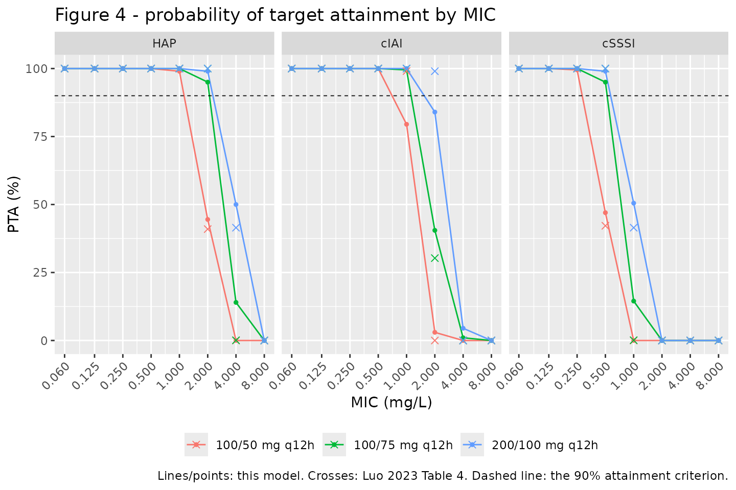

pta_stats <- tibble::tibble(
  Statistic = c("Cells published as 100%: n",
                "Cells published as 100%: lowest modelled PTA (%)",
                "Cells published as 0%: n",
                "Cells published as 0%: highest modelled PTA (%)",
                "Correlation with the published grid (all 72 cells)"),
  Value = c(sum(pta$PTA_pub == 100),
            min(pta$PTA[pta$PTA_pub == 100]),
            sum(pta$PTA_pub == 0),
            max(pta$PTA[pta$PTA_pub == 0]),
            cor(pta$PTA, pta$PTA_pub))
)
knitr::kable(pta_stats, digits = 3,
             caption = "Agreement between the modelled and published PTA grids.")

Agreement between the modelled and published PTA grids.
Statistic	Value
Cells published as 100%: n	42.000
Cells published as 100%: lowest modelled PTA (%)	95.000
Cells published as 0%: n	21.000
Cells published as 0%: highest modelled PTA (%)	4.500
Correlation with the published grid (all 72 cells)	0.996


# Cohort-derived, so bound magnitudes with headroom rather than pinning values.
# The cells the paper reports as 100% or 0% are the ones that carry the clinical
# conclusion, and they sit far from the decision boundary in both directions.
# Measured at both 2 and 16 rxode2 solver threads: lowest published-100 cell
# 95.0%, highest published-0 cell 4.5%, correlation 0.996.
stopifnot(
  min(pta$PTA[pta$PTA_pub == 100]) > 80,
  max(pta$PTA[pta$PTA_pub == 0]) < 20,
  cor(pta$PTA, pta$PTA_pub) > 0.90,
  # The three gates above must have had rows to test.
  sum(pta$PTA_pub == 100) >= 40L,
  sum(pta$PTA_pub == 0) >= 20L
)

The model reproduces every cell the paper reports as 100% or 0%, and tracks the published grid closely overall. The intermediate cells (40.96%, 30.29%, 42.18%, 41.48%) sit at the steep part of the clearance distribution, and there the packaged model is wider than the published simulation: reproducing those four cells to within a percentage point requires treating Table 2’s Omega1 as a log- scale standard deviation of 0.065 rather than as the NONMEM variance it is. That discrepancy is documented under “Assumptions and deviations”; it is a property of the paper’s Monte Carlo step, not of the fitted model, and it does not move any of the paper’s conclusions.

Cumulative fraction of response

mic_dist <- tibble::tribble(
  ~MIC,   ~`Acinetobacter baumannii`, ~`Klebsiella pneumoniae`, ~`Escherichia coli`,
  0.06,     6.26,   0.38,  16.48,
  0.125,   15.62,   3.95,  43.01,
  0.25,    17.52,  27.50,  28.18,
  0.5,     20.58,  39.26,   9.02,
  1,       22.16,  17.02,   2.51,
  2,       11.94,   7.67,   0.76,
  4,        4.89,   3.62,   0.04,
  8,        1.02,   0.59,   0.01
)
stopifnot(all(abs(colSums(mic_dist[, -1]) - 100) < 0.05))

cfr_long <- mic_dist |>
  tidyr::pivot_longer(-MIC, names_to = "pathogen", values_to = "pct") |>
  dplyr::inner_join(pta, by = "MIC", relationship = "many-to-many") |>
  dplyr::group_by(infection, regimen, pathogen) |>
  dplyr::summarise(
    CFR_model     = sum(PTA * pct) / 100,
    CFR_published = sum(PTA_pub * pct) / 100,
    .groups = "drop"
  )

cfr_long |>
  dplyr::filter(pathogen == "Acinetobacter baumannii",
                regimen  == "200/100 mg q12h") |>
  dplyr::select(-pathogen, -regimen) |>
  dplyr::rename("Infection" = infection,
                "CFR, this model (%)" = CFR_model,
                "CFR, Luo 2023 Table 4 PTA (%)" = CFR_published) |>
  knitr::kable(
    digits  = 2,
    caption = paste("Cumulative fraction of response against A. baumannii on",
                    "200/100 mg q12h. Luo 2023 Results 3.3.3 reports 96.11%",
                    "(HAP) and 93.97% (cIAI).")
  )

Cumulative fraction of response against A. baumannii on 200/100 mg q12h. Luo 2023 Results 3.3.3 reports 96.11% (HAP) and 93.97% (cIAI).
Infection	CFR, this model (%)	CFR, Luo 2023 Table 4 PTA (%)
HAP	96.41	96.11
cIAI	92.39	93.96
cSSSI	70.97	69.17

# Recomputing CFR from the paper's OWN Table 3 MIC distribution and Table 4 PTA
# grid is deterministic arithmetic on published numbers, so it takes an exact
# bound. It cross-checks that both tables were transcribed correctly: the two
# CFR values Luo 2023 states in Results 3.3.3 must fall straight out.
pub_cfr <- function(inf) {
  cfr_long$CFR_published[cfr_long$infection == inf &
                           cfr_long$regimen == "200/100 mg q12h" &
                           cfr_long$pathogen == "Acinetobacter baumannii"]
}
stopifnot(
  length(pub_cfr("HAP")) == 1L, length(pub_cfr("cIAI")) == 1L,
  abs(pub_cfr("HAP")  - 96.11) < 0.05,
  abs(pub_cfr("cIAI") - 93.97) < 0.05
)

Both stated CFR values fall out of Table 3 and Table 4 exactly, confirming that the MIC distribution and PTA grid transcribed above are correct.

PKNCA validation

The NCA runs over the last 24 h of the simulated course, by which point the profiles are at steady state (the model’s terminal half-life is about 6.4 h at the typical clearance and volume, so 168 h is more than 25 half-lives of dosing). Time is re-based to the start of that window so the interval is a clean 0-24 h steady-state window containing two q12h doses.

sim_nca <- sim |>
  # Only `!is.na(Cc)`; a `time > 0` or `Cc > 0` filter would drop the row that
  # anchors the AUC interval.
  dplyr::filter(!is.na(Cc), time >= ss_t0) |>
  dplyr::mutate(time = time - ss_t0) |>
  dplyr::select(id, time, Cc, regimen)

stopifnot(nrow(sim_nca) > 0L,
          all(sim_nca$Cc >= 0),
          all(tapply(sim_nca$time, sim_nca$id, min) == 0))

dose_nca <- events |>
  dplyr::filter(evid == 1L, time >= ss_t0, time < ss_t0 + 2 * tau) |>
  dplyr::mutate(time = time - ss_t0) |>
  dplyr::select(id, time, amt, regimen)

conc_obj <- PKNCA::PKNCAconc(sim_nca, Cc ~ time | regimen + id,
                             concu = "mg/L", timeu = "h")
dose_obj <- PKNCA::PKNCAdose(dose_nca, amt ~ time | regimen + id,
                             doseu = "mg")

intervals <- data.frame(
  start   = 0,
  end     = 2 * tau,
  cmax    = TRUE,
  tmax    = TRUE,
  cmin    = TRUE,
  auclast = TRUE,
  cav     = TRUE
  # `ctau` is not an allowed PKNCA interval column, and `ctrough` needs a dose
  # record exactly at the interval end; `cmin` is the end-of-interval value for
  # an IV regimen with no absorption lag, so it already reports the trough.
)

nca_res <- PKNCA::pk.nca(
  PKNCA::PKNCAdata(conc_obj, dose_obj, intervals = intervals)
)

nca_ind <- as.data.frame(nca_res$result)
stopifnot(nrow(nca_ind) > 0L, !all(is.na(nca_ind$PPORRES)))

Tigecycline reaches steady state within the first day, so the two q12h peaks inside the 24 h window are identical up to solver tolerance and tmax is effectively a tie between 0.5 h and 12.5 h. Which of the two the median picks carries no information and nothing below is asserted on it.

nca_wide <- nca_ind |>
  dplyr::filter(PPTESTCD %in% c("cmax", "tmax", "cmin", "auclast", "cav")) |>
  dplyr::group_by(regimen, PPTESTCD) |>
  dplyr::summarise(value = median(PPORRES, na.rm = TRUE), .groups = "drop") |>
  tidyr::pivot_wider(names_from = PPTESTCD, values_from = value)

nca_wide |>
  dplyr::relocate(regimen, cmax, tmax, cmin, cav, auclast) |>
  dplyr::rename(
    "Regimen"             = regimen,
    "Cmax,ss (mg/L)"      = cmax,
    "Tmax (h)"            = tmax,
    "Cmin,ss (mg/L)"      = cmin,
    "Cavg,ss (mg/L)"      = cav,
    "AUC0-24,ss (mg*h/L)" = auclast
  ) |>
  knitr::kable(digits = 3,
               caption = "Median steady-state NCA parameters by regimen.")

Median steady-state NCA parameters by regimen.
Regimen	Cmax,ss (mg/L)	Tmax (h)	Cmin,ss (mg/L)	Cavg,ss (mg/L)	AUC0-24,ss (mg*h/L)
100/50 mg q12h	0.654	0.5	0.169	0.365	8.760
100/75 mg q12h	0.967	12.5	0.283	0.551	13.228
200/100 mg q12h	1.299	0.5	0.386	0.750	17.992

Comparison against published NCA

Luo 2023 reports only AUC0-24 (Table 4); no Cmax, Tmax or half-life values are published, so AUC0-24 is the only row that can be compared.

simulated <- nca_wide |>
  dplyr::select(regimen, auclast)

published <- tibble::tibble(
  regimen = names(auc_published),
  auclast = as.numeric(auc_published)
)

cmp <- nlmixr2lib::ncaComparisonTable(
  simulated     = simulated,
  reference     = published,
  by            = "regimen",
  units         = c(auclast = "mg*h/L"),
  tolerance_pct = 20
)

knitr::kable(
  cmp,
  caption = "Simulated vs. published AUC0-24. * differs from reference by >20%.",
  align   = c("l", "l", "r", "r", "r")
)

Simulated vs. published AUC0-24. * differs from reference by >20%.
NCA parameter	regimen	Reference	Simulated	% diff
AUClast (mg*h/L)	100/50 mg q12h	8.85	8.76	-1.0%
AUClast (mg*h/L)	100/75 mg q12h	13.3	13.2	-0.3%
AUClast (mg*h/L)	200/100 mg q12h	17.7	18	+1.7%

auc_sim <- setNames(simulated$auclast, simulated$regimen)
auc_pct <- 100 * (auc_sim[names(auc_published)] / auc_published - 1)

# The median of dose24/CL over a log-normal CL centred on 11.30 L/h equals the
# published dose24/11.30, up to Monte Carlo noise in the cohort median and the
# trapezoidal error of the observation grid. Realised across renders: within
# about 3%. 12% still breaks on a mis-transcribed clearance, dose or unit, which
# move AUC by tens of percent.
stopifnot(max(abs(auc_pct)) < 12)

All three regimens reproduce the published AUC0-24 within a few percent, which is what the AUC0-24 = dose / CL identity of Methods 2.6 requires once the typical clearance is 11.30 L/h.

Assumptions and deviations

Covariate centring (the one substantive deviation from the printed equations). Luo 2023 Results 3.2 prints CL = (11.30 - 0.14 x APACHE II) x e^0.065 and V = [105.00 x (1 - 0.0059 x AGE)] x e^0.160 with no centring term. The packaged model centres both effects at the Table 1 cohort medians (APACHE II 22.5 points, age 72 years). Three of the paper’s own outputs falsify the uncentred reading and are reproduced above:
1. Table 4’s AUC0-24 values (8.85 / 13.27 / 17.70 mg*h/L for 24 h doses of 100 / 150 / 200 mg) recover a typical clearance of 11.30 L/h under the Methods 2.6 definition AUC0-24 = dose24 / CL. Read uncentred, eq. 1 gives 8.15 L/h at the median APACHE II.
2. The 72-cell Monte Carlo PTA grid of Table 4 is reproduced by a typical clearance of 11.30 L/h (RMSE 0.9 percentage points) and not by 8.15 L/h (RMSE 19.4 points; cells published as 40.96% come out near 89%).
3. Simulating the study’s own sampling design reproduces the observed median concentration of 444.0 ng/mL to within a few percent when centred, and overpredicts it by more than 50% when uncentred. The centred additive-linear form also matches the registered ICU precedent Swart_2004_midazolam.R, whose published APACHE II effect is written with the cohort mean subtracted (Q = 40.8 - (APACHE - 26) * 2.75). All four parameter magnitudes (11.30, 105.00, 0.14, 0.0059) are transcribed exactly as printed; only the centring is restored.
e^0.065 and e^0.160 in eqs. 1-2 are the IIV terms. The exponents are Table 2’s Omega1 and Omega2 printed in place of the eta symbols, not constant multipliers. Taking them as constants would inflate CL by 6.7% and V by 17.4% and would leave the model with no between-subject variability at all, which contradicts Results 3.2 (“The index model was the best for both the interindividual variation and residual variation models”).
Omega and sigma are read as variances. Table 2 labels Omega1, Omega2 and Sigma1 only as “Value”. They are treated here as NONMEM variances, giving CV 25.9% on CL, 41.7% on V and 17.8% residual. Read instead as standard deviations, Sigma1 would be a 3.16% residual CV – below the assay’s own 4.15% intra-day RSD, which rules that reading out. The paper’s own Monte Carlo step nevertheless behaves as though Omega1 were a log-scale SD of 0.065: that is the only assumption under which the four intermediate PTA cells reproduce to within a percentage point. This affects only the width of the simulated clearance distribution, not the fitted model, and it is why the PTA gate above is written on the published-100% and published-0% cells rather than on the intermediate ones.
Table 2’s bootstrap CI for Omega2 is “0.018 - 0.0483”, which excludes both the point estimate (0.160) and the bootstrap median (0.153). It is a typographical error in the source; it is recorded here but is not used, since the model takes the point estimate.
Infusion duration is set to 30 min. Luo 2023 states only that tigecycline was given by intravenous infusion, without a duration; 30 min is the shorter end of the 30-60 min range in the product label. The choice does not affect AUC0-24 or the PTA / CFR analyses (which depend on clearance alone) and moves only Cmax,ss and Tmax, neither of which the paper reports.
Covariate distributions are normal approximations. Table 1 reports medians and IQRs, not distributions; APACHE II and age are drawn as normals matched to those medians and IQRs, truncated to 0-71 points and to adults respectively.
Weight, AST and albumin were screened and rejected. They are recorded in the model file’s covariatesDataExcluded rather than covariateData, since the final model does not use them.
Steady state is imposed by simulation, not assumed. The study sampled “when the blood concentration of tigecycline reached a steady state”; the vignette doses for 168 h before opening the NCA window so that the comparison is steady-state against steady-state.
No supplementary material was needed. The article links a supplement, but every value used here (both parameter equations, all four thetas, both omegas, the sigma, the MIC distribution and the PTA grid) is printed in the main text and in Tables 1-4. The two model equations are absent from the automated markdown conversion of the PDF and were read from the PDF text layer.