Morphine brain distribution in the rat (Groenendaal 2007)
Source:vignettes/articles/Groenendaal_2007_morphine_brain_rat.Rmd
Groenendaal_2007_morphine_brain_rat.Rmd
mod <- rxode2::rxode(readModelDb("Groenendaal_2007_morphine_brain_rat"))
#> ℹ parameter labels from comments will be replaced by 'label()'
Model and source
- Citation: Groenendaal D, Freijer J, de Mik D, Bouw MR, Danhof M, de Lange ECM. Population pharmacokinetic modelling of non-linear brain distribution of morphine: influence of active saturable influx and P-glycoprotein mediated efflux. Br J Pharmacol. 2007;151(5):701-712. doi:10.1038/sj.bjp.0707257.
- Article: https://doi.org/10.1038/sj.bjp.0707257
- PubMed Central: https://www.ncbi.nlm.nih.gov/pmc/articles/PMC2014001/
- Companion paper (separate model, not extracted here): Groenendaal
et al.
- Br J Pharmacol 151(4):713-720, https://doi.org/10.1038/sj.bjp.0707258 – the EEG PK-PD biophase model fitted to the same experiments.
Preclinical (rat, male Wistar). Non-linear blood-brain barrier (BBB) distribution model for morphine published by Groenendaal et al. (2007, Br J Pharmacol 151(5):701-712). A three-compartment blood disposition model (paper Table 2, NONMEM ADVAN11 TRANS4; linear body-weight effects on CL and on the first peripheral volume V2) drives a single brain extracellular-fluid (ECF) compartment sampled by intracerebral striatal microdialysis. Mass exchange across the BBB is split into three explicit terms (paper equations 9-11): bidirectional passive diffusion kdiff * (Cblood - Cecf), a saturable active influx Nmax Cblood / (C50 + Cblood) that is already near-saturated at the lowest studied dose, and an active P-glycoprotein-mediated efflux keff * Cecf. Co-infusion of the Pgp inhibitor GF120918 (elacridar) lowers keff from 0.0195 to 0.0113 1/min (a 42% reduction) and leaves kdiff, Nmax and C50 unchanged; the blood disposition is unaffected by GF120918. Inter-animal variability is on CL, V2, kdiff and keff, with a kdiff-keff covariance block (paper Table 3). Because the paper reports the volume-aggregated brain parameters (kdiff = Qdiff/Vecf, Nmax = Nmax/Vecf, keff = Qeff/Vecf) and never identifies Vecf itself, the brain_ecf state carries a concentration (ng/mL) rather than an amount; see the validation vignette for the dimensional argument.
Population
The model was built from a single rat study at Leiden University (paper Table 1). Seventy-one male Wistar rats (Charles River, Maastricht), 250-350 g, received a 10 min zero-order intravenous infusion of morphine hydrochloride at 4, 10 or 40 mg/kg. The 4 mg/kg level was studied both with vehicle and with a co-infusion of the P-glycoprotein inhibitor GF120918 (elacridar); 10 and 40 mg/kg were vehicle only. All animals received a continuous midazolam infusion (5.5 mg/kg/h) to suppress opioid-induced seizure activity, and animals in the 40 mg/kg arm were artificially ventilated with vecuronium-bromide muscle relaxation because of severe respiratory depression.
The two model layers were fitted sequentially in NONMEM V (FOCE INTERACTION). The blood three-compartment layer used arterial blood morphine from all 71 animals (15 samples per rat to 360 min). The brain layer used recovery-corrected striatal microdialysate from the 32 animals perfused with blank perfusate – the 50 and 500 ng/mL retrodialysis animals yielded no usable post-dose ECF data and were excluded (paper Microdialysis probe recovery).
The same information is available programmatically:
str(mod$population)
#> List of 11
#>  $ species       : chr "rat (male Wistar, Charles River, Maastricht, The Netherlands)"
#>  $ n_subjects    : int 71
#>  $ n_studies     : int 1
#>  $ age_range     : chr "adult (age not reported; animals housed at least 7 days after arrival, then 10 days of recovery after electrode"| __truncated__
#>  $ weight_range  : chr "250-350 g body weight; per-group means 0.260-0.306 kg (paper Table 1)"
#>  $ sex_female_pct: num 0
#>  $ race_ethnicity: logi NA
#>  $ disease_state : chr "Healthy rats prepared with four indwelling cannulas (right femoral artery for serial arterial blood sampling; b"| __truncated__
#>  $ dose_range    : chr "Single 10 min zero-order intravenous infusion of morphine hydrochloride in saline at 4, 10 or 40 mg/kg. The 4 m"| __truncated__
#>  $ regions       : chr "preclinical (in-vivo rat); Leiden University, The Netherlands"
#>  $ notes         : chr "Two model layers, fitted sequentially in NONMEM V level 1.1 with FOCE INTERACTION. (1) The blood three-compartm"| __truncated__
Model structure
The blood layer is an ordinary three-compartment disposition model
(NONMEM ADVAN11 TRANS4), with body weight entering CL and
the first peripheral volume V2 through the paper’s centred
linear covariate form (equation 7),
which is a linear slope in kg, not an allometric power.
The brain layer is the paper’s contribution. Equation 9 writes the mass balance on the amount of morphine in brain extracellular fluid as three explicit transport terms,
and equations 10-11 divide through by the brain ECF distribution volume and name the aggregated constants , and :
is never identified, so every published brain parameter is already
volume-aggregated. The packaged model therefore carries
brain_ecf as a concentration state in
ng/mL rather than an amount – encoding an amount would require inventing
.
The mechanism the paper is after: with ng/mL, the active influx is essentially saturated at every blood concentration the study produced, so it behaves as a constant input of . As the dose rises, that fixed contribution is diluted by the dose-proportional passive term, and the dose-normalised brain exposure falls.
Source trace
Every equation and every ini() value, with its location
in the paper.
| Item | Value | Source |
|---|---|---|
| Blood disposition structure | 3-compartment, ADVAN11 TRANS4 | Methods, PK analysis of blood profiles |
| Body-weight covariate form | P = t1 * (1 + t2 * (BW - median BW)) | Equation 7 |
| GF120918 covariate form | P = t3 * (1 - GF) + t4 * GF | Equation 8 |
| Brain ECF mass balance | dAecf/dt, three transport terms | Equation 9 |
| Brain ECF concentration form | dCecf/dt after dividing by Vecf | Equation 10 |
| Parameter aggregation | kdiff, N*max, keff = Q../Vecf | Equation 11 |
| IIV form | P_i = P_typ * exp(eta), eta ~ N(0, omega^2) | Equations 3-4 |
| Residual error form | Cobs = Cpred * (1 + eps), eps ~ N(0, sigma^2) | Equations 5-6 |
| lcl = log(20.0) | Cl Intercept 20.0 mL/min (CV 5.6%) | Table 2 |
| e_wt_cl = 5.35 | Cl Slope factor 5.35 /kg (CV 25.2%) | Table 2 |
| lvc = log(68.1) | V1 68.1 mL (CV 16.7%) | Table 2 |
| lq = log(15.5) | Q2 15.5 mL/min (CV 11.3%) | Table 2 |
| lvp = log(739) | V2 Intercept 739 mL (CV 7.6%) | Table 2 |
| e_wt_vp = 8.50 | V2 Slope factor 8.50 /kg (CV 17.1%) | Table 2 |
| lq2 = log(17.8) | Q3 17.8 mL/min (CV 18.4%) | Table 2 |
| lvp2 = log(133) | V3 133 mL (CV 15.9%) | Table 2 |
| etalcl ~ 0.129 | omega^2 Cl 0.129 (CV 17.2%) | Table 2 |
| etalvp ~ 0.099 | omega^2 V2 0.099 (CV 24.7%) | Table 2 |
| propSd = sqrt(0.074) | Proportional error 0.074 (CV 10.2%) | Table 2 |
| lkdiff_bbb = log(0.0014) | kdiff 0.0014 /min (CV 12.6%) | Table 3 |
| lkefflux_bbb = log(0.0195) | keff -GF120918 0.0195 /min (CV 12.2%) | Table 3 |
| e_conmed_elacridar_kefflux_bbb | keff +GF120918 0.0113 /min (CV 25.4%) | Table 3 |
| lNstarMax = log(0.658) | N*max 0.658 ng/mL/min (CV 26.1%) | Table 3 (units per Abstract) |
| lc50 = log(9.92) | C50 9.92 ng/mL (CV 71.5%) | Table 3 |
| etalkdiff_bbb / etalkefflux_bbb block | 0.238 / cov 0.059 / 0.080 | Table 3 |
| propSd_Cbrain_ecf = sqrt(0.094) | Proportional error 0.094 (CV 21.4%) | Table 3 |
Virtual cohort
Three arms matching the paper’s brain-ECF design, 30 rats each. Body weights are drawn uniformly over the paper’s stated 250-350 g range (the paper reports only the range and per-group means, not the individual weights).
rxode2::rxSetSeed(20070430)

REF_WT   <- 0.300      # kg; stands in for the paper's unprinted `median BW`
N_PER_ARM <- 30L       # well under the 200-per-arm cap

arms <- tibble::tribble(
  ~arm,                  ~dose_mgkg, ~gf,
  "4 mg/kg vehicle",              4,   0,
  "4 mg/kg + GF120918",           4,   1,
  "40 mg/kg vehicle",            40,   0
) |>
  mutate(arm = factor(arm, levels = arm))

subj <- arms |>
  tidyr::crossing(subj_no = seq_len(N_PER_ARM)) |>
  mutate(
    id = dplyr::row_number(),
    WT = runif(dplyr::n(), min = 0.250, max = 0.350),
    CONMED_ELACRIDAR = gf,
    amt = dose_mgkg * WT * 1e6      # ng
  )

# Observation grid: dense through the infusion and distribution phase, then
# every 15 min to 360 min. 165 min is included explicitly because the paper's
# dose-normalised AUC is reported over 0-165 min.
obs_times <- sort(unique(c(
  0, 1, 2, 3, 5, 7.5, 10, 12, 15, 20, 25, 30, 40, 50, 60,
  seq(75, 360, by = 15), 165
)))
The two observables are separate nlmixr2 endpoints (Cc
is endpoint 1, Cbrain_ecf endpoint 2), so every observation
row carries a dvid. The row is addressed at the real ODE
state central; rxode2 maps dvid 1 and 2 onto
the endpoint pseudo-compartments it appended after the four ODE states,
which the solved output reports as CMT 5 and 6.
dose_rows <- subj |>
  transmute(id, arm, WT, CONMED_ELACRIDAR,
            time = 0, amt, rate = amt / 10,   # 10 min zero-order infusion
            evid = 1L, cmt = "central", dvid = NA_integer_)

obs_rows <- subj |>
  select(id, arm, WT, CONMED_ELACRIDAR) |>
  tidyr::crossing(time = obs_times, dvid = 1:2) |>
  mutate(amt = NA_real_, rate = NA_real_, evid = 0L, cmt = "central")

events <- bind_rows(dose_rows, obs_rows[names(dose_rows)]) |>
  arrange(id, time, dvid)
Simulation
sim <- rxode2::rxSolve(
  mod, events,
  keep = c("arm", "WT", "CONMED_ELACRIDAR"),
  useLinCmt = FALSE,           # ODE -> linCmt auto-conversion breaks dvid mapping
  returnType = "data.frame"
) |>
  as_tibble()

# CMT 5 rows are the Cc endpoint, CMT 6 rows the Cbrain_ecf endpoint; `sim`
# carries the residual error for whichever endpoint the row belongs to, while
# Cc / Cbrain_ecf are the individual predictions.
blood <- sim |>
  filter(CMT == min(CMT)) |>
  # `cl` is the solver's own INDIVIDUAL clearance for this subject (typical
  # value * exp(etalcl) * the body-weight factor); it is what the blood
  # identity check below must be compared against.
  transmute(id, arm, WT, time, cl, ipred = Cc, obs = sim)

ecf <- sim |>
  filter(CMT == max(CMT)) |>
  transmute(id, arm, WT, time, ipred = Cbrain_ecf, obs = sim)

nrow(blood)
#> [1] 3150
nrow(ecf)
#> [1] 3150
Typical-value (no IIV, no residual error) profiles at the reference weight, used for every deterministic check below.
typ_events <- arms |>
  mutate(id = dplyr::row_number(), WT = REF_WT,
         CONMED_ELACRIDAR = gf, amt = dose_mgkg * REF_WT * 1e6) |>
  select(id, arm, WT, CONMED_ELACRIDAR, amt, dose_mgkg)

typ_dose <- typ_events |>
  transmute(id, arm, WT, CONMED_ELACRIDAR, time = 0, amt, rate = amt / 10,
            evid = 1L, cmt = "central", dvid = NA_integer_)

typ_obs <- typ_events |>
  select(id, arm, WT, CONMED_ELACRIDAR) |>
  tidyr::crossing(time = sort(unique(c(seq(0, 360, by = 0.5), 165))), dvid = 1:2) |>
  mutate(amt = NA_real_, rate = NA_real_, evid = 0L, cmt = "central")

typ_sim <- rxode2::rxSolve(
  mod,
  bind_rows(typ_dose, typ_obs[names(typ_dose)]) |> arrange(id, time, dvid),
  keep = c("arm", "WT", "CONMED_ELACRIDAR"),
  omega = NA, sigma = NA, useLinCmt = FALSE, returnType = "data.frame"
) |>
  as_tibble() |>
  filter(CMT == min(CMT)) |>
  transmute(arm, time, Cc, Cbrain_ecf) |>
  left_join(select(typ_events, arm, dose_mgkg), by = "arm")
Replicating the published figures
Figure 2 – morphine in blood
blood_q <- blood |>
  group_by(arm, time) |>
  summarise(lo = quantile(obs, 0.025), hi = quantile(obs, 0.975), .groups = "drop")

ggplot(blood, aes(time, obs)) +
  geom_point(colour = "grey60", size = 0.5, alpha = 0.5) +
  geom_ribbon(data = blood_q, aes(time, ymin = pmax(lo, 1), ymax = hi),
              inherit.aes = FALSE, alpha = 0.2) +
  geom_line(data = typ_sim, aes(time, Cc), linewidth = 0.8) +
  annotate("rect", xmin = 0, xmax = 10, ymin = 1, ymax = Inf, alpha = 0.15) +
  facet_wrap(~arm) +
  scale_y_log10() +
  coord_cartesian(xlim = c(0, 360)) +
  labs(x = "Time (min)", y = "Morphine in blood (ng/mL)")
#> Warning in scale_y_log10(): log-10 transformation introduced infinite values.
#> log-10 transformation introduced infinite values.
#> log-10 transformation introduced infinite values.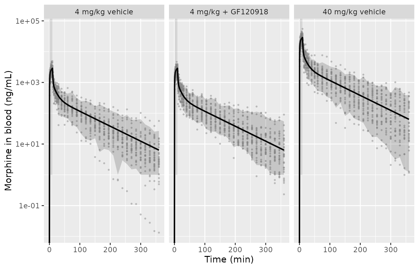
Replicates Figure 2 of Groenendaal 2007: simulated morphine blood concentrations by dose group. Points are simulated observations (individual prediction plus proportional residual error), the solid line the typical-value prediction, the ribbon the 2.5-97.5% simulated interval.
Figure 3 / 6 – morphine in brain ECF
ecf_q <- ecf |>
  group_by(arm, time) |>
  summarise(lo = quantile(obs, 0.025), hi = quantile(obs, 0.975), .groups = "drop")

ggplot(ecf, aes(time, obs)) +
  geom_point(colour = "grey60", size = 0.5, alpha = 0.5) +
  geom_ribbon(data = ecf_q, aes(time, ymin = pmax(lo, 0), ymax = hi),
              inherit.aes = FALSE, alpha = 0.2) +
  geom_line(data = typ_sim, aes(time, Cbrain_ecf), linewidth = 0.8) +
  annotate("rect", xmin = 0, xmax = 10, ymin = 0, ymax = Inf, alpha = 0.15) +
  facet_wrap(~arm, scales = "free_y") +
  labs(x = "Time (min)", y = "Morphine in brain ECF (ng/mL)")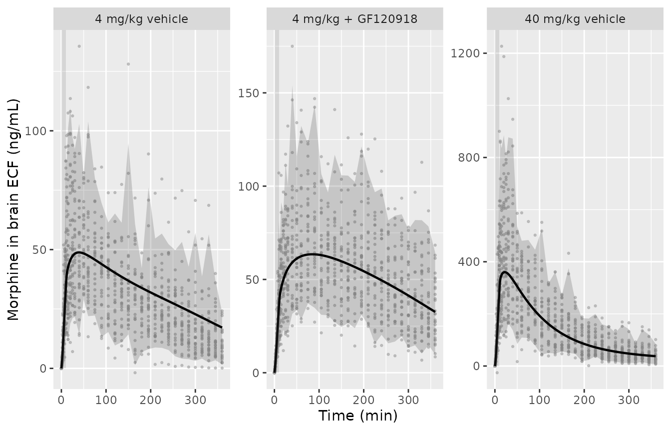
Replicates Figures 3 and 6 of Groenendaal 2007: simulated brain ECF morphine concentrations by dose group, with the typical-value prediction and the 2.5-97.5% simulated interval. The 4 mg/kg arms reach a near-plateau; the 40 mg/kg arm declines clearly after its early peak.
Figure 4 – dose-normalised brain ECF
Normalising to the 4 mg/kg dose makes the non-linearity explicit: if brain distribution were linear, the three curves would superimpose.
ggplot(typ_sim, aes(time, Cbrain_ecf * 4 / dose_mgkg, colour = arm)) +
  geom_line(linewidth = 0.8) +
  annotate("rect", xmin = 0, xmax = 10, ymin = 0, ymax = Inf, alpha = 0.15) +
  labs(x = "Time (min)", y = "Dose-normalised brain ECF (ng/mL per 4 mg/kg)",
       colour = NULL) +
  theme(legend.position = "bottom")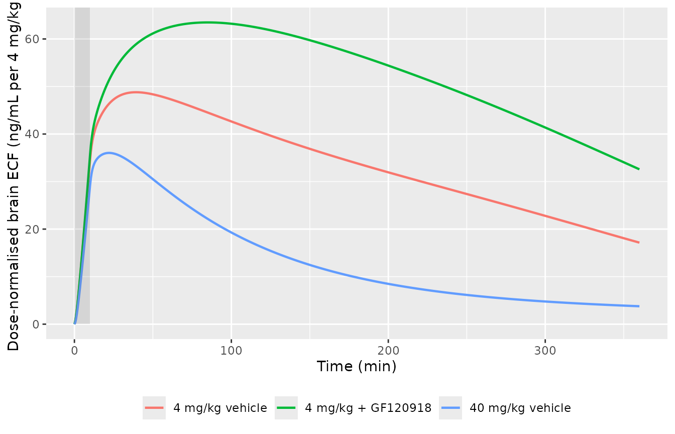
Replicates Figure 4 of Groenendaal 2007: brain ECF concentrations normalised to a 4 mg/kg dose. The 40 mg/kg profile sits well below the 4 mg/kg profiles over most of the interval, the signature of a saturable active influx.
Figure 5 – simulated dose range
dose_grid <- tidyr::crossing(dose_mgkg = c(4, 10, 20, 40), gf = c(0, 1)) |>
  mutate(id = dplyr::row_number(), WT = REF_WT, CONMED_ELACRIDAR = gf,
         amt = dose_mgkg * REF_WT * 1e6,
         label = paste0(dose_mgkg, " mg/kg"),
         pgp = ifelse(gf == 1, "+ GF120918", "vehicle"))

dg_dose <- dose_grid |>
  transmute(id, label, pgp, WT, CONMED_ELACRIDAR, time = 0, amt, rate = amt / 10,
            evid = 1L, cmt = "central", dvid = NA_integer_)
dg_obs <- dose_grid |>
  select(id, label, pgp, WT, CONMED_ELACRIDAR) |>
  tidyr::crossing(time = seq(0, 360, by = 2), dvid = 1:2) |>
  mutate(amt = NA_real_, rate = NA_real_, evid = 0L, cmt = "central")

dg_sim <- rxode2::rxSolve(
  mod, bind_rows(dg_dose, dg_obs[names(dg_dose)]) |> arrange(id, time, dvid),
  keep = c("label", "pgp"), omega = NA, sigma = NA,
  useLinCmt = FALSE, returnType = "data.frame"
) |>
  as_tibble() |>
  filter(CMT == min(CMT))

ggplot(dg_sim, aes(time, Cbrain_ecf, colour = label)) +
  geom_line(linewidth = 0.8) +
  facet_wrap(~pgp) +
  labs(x = "Time (min)", y = "Morphine in brain ECF (ng/mL)", colour = "Dose") +
  theme(legend.position = "bottom")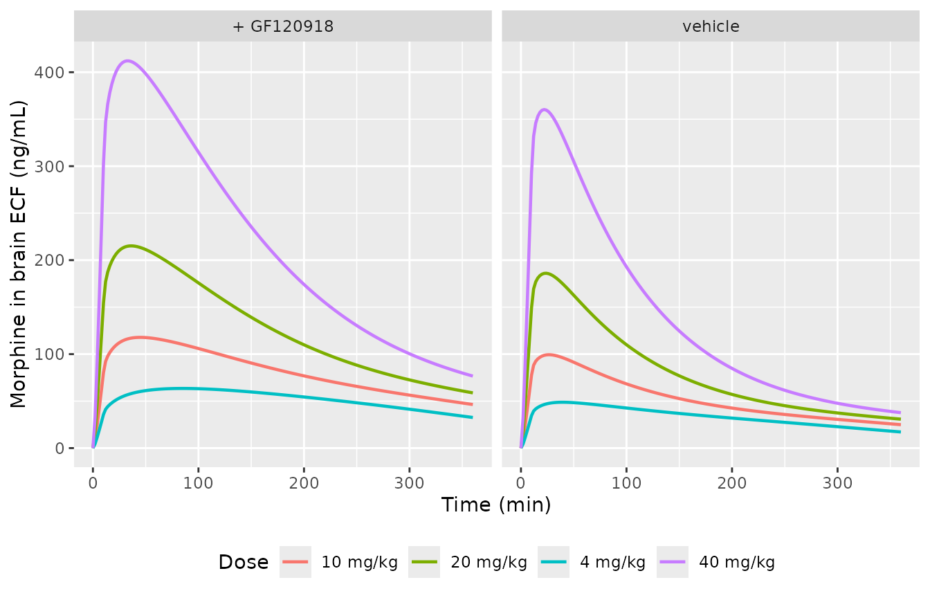
Replicates Figure 5 of Groenendaal 2007: typical-value brain ECF profiles across the 4-40 mg/kg dose range with and without GF120918. Stable plateau concentrations at low dose give way to a clear decline as dose increases.
PKNCA validation
NCA is run on the individual predictions (rather than on the residual-error simulated observations) so the log-down trapezoid never sees a negative concentration. The paper’s comparator is a group mean, and the summary here is the cohort median.
dose_df <- subj |>
  transmute(id, arm, time = 0, amt)

# Blood
conc_blood <- blood |>
  filter(!is.na(ipred)) |>
  transmute(id, arm, time, Cc = ipred)

blood_obj <- PKNCA::PKNCAconc(conc_blood, Cc ~ time | arm + id,
                              concu = "ng/mL", timeu = "min")
dose_obj  <- PKNCA::PKNCAdose(dose_df, amt ~ time | arm + id, doseu = "ng")

blood_res <- PKNCA::pk.nca(PKNCA::PKNCAdata(
  blood_obj, dose_obj,
  intervals = data.frame(start = 0, end = Inf,
                         cmax = TRUE, tmax = TRUE, auclast = TRUE,
                         aucinf.obs = TRUE, half.life = TRUE, cl.obs = TRUE)
))
summary(blood_res)
#>  Interval Start Interval End                arm  N AUClast (min*ng/mL)
#>               0          Inf    4 mg/kg vehicle 30        55700 [42.3]
#>               0          Inf 4 mg/kg + GF120918 30        63400 [39.0]
#>               0          Inf   40 mg/kg vehicle 30       625000 [34.0]
#>  Cmax (ng/mL)        Tmax (min) Half-life (min) AUCinf,obs (min*ng/mL)
#>   2710 [17.3] 10.0 [10.0, 10.0]     59.6 [22.3]           56400 [43.8]
#>   2910 [16.4] 10.0 [10.0, 10.0]     70.4 [25.6]           64700 [40.2]
#>  28800 [13.9] 10.0 [10.0, 10.0]     69.2 [26.9]          638000 [36.1]
#>  CL (based on AUCinf,obs) (ng/(min*ng/mL))
#>                                20.9 [50.9]
#>                                18.4 [44.2]
#>                                18.4 [39.7]
#>
#> Caption: AUClast, Cmax, AUCinf,obs, CL (based on AUCinf,obs): geometric mean and geometric coefficient of variation; Tmax: median and range; Half-life: arithmetic mean and standard deviation; N: number of subjects
conc_ecf <- ecf |>
  filter(!is.na(ipred)) |>
  transmute(id, arm, time, Cc = ipred)

ecf_obj <- PKNCA::PKNCAconc(conc_ecf, Cc ~ time | arm + id,
                            concu = "ng/mL", timeu = "min")

# The paper's brain-ECF exposure metric is AUC over the largest common
# interval, 0-165 min.
ecf_res <- PKNCA::pk.nca(PKNCA::PKNCAdata(
  ecf_obj, dose_obj,
  intervals = data.frame(start = 0, end = 165,
                         cmax = TRUE, tmax = TRUE, auclast = TRUE)
))
summary(ecf_res)
#>  Interval Start Interval End                arm  N AUClast (min*ng/mL)
#>               0          165    4 mg/kg vehicle 30         6850 [33.7]
#>               0          165 4 mg/kg + GF120918 30        10500 [33.9]
#>               0          165   40 mg/kg vehicle 30        37400 [44.2]
#>  Cmax (ng/mL)        Tmax (min)
#>   54.4 [39.6]  30.0 [15.0, 150]
#>   75.9 [37.7]  75.0 [25.0, 165]
#>    365 [48.4] 25.0 [15.0, 40.0]
#>
#> Caption: AUClast, Cmax: geometric mean and geometric coefficient of variation; Tmax: median and range; N: number of subjects
Blood: an exact internal identity
For a linear disposition model, AUC(0-inf) in blood must equal
Dose/CL exactly, and PKNCA’s cl.obs must return the
subject’s own clearance. Both sides of this comparison come from the
same simulated subject – cl.obs is
Dose / AUCinf.obs computed from that subject’s profile, and
cl is the individual clearance the solver used to generate
it – so the only thing separating them is trapezoidal and lambda-z error
on the sampling grid. There is no cohort randomness in the difference,
which is why it is asserted tightly.
The comparison must use the individual clearance,
not the typical value: IIV on CL is omega^2 = 0.129 (a ~36%
CV on the log scale), so comparing NCA clearance against the
typical-value CL differs by exp(etalcl) and spreads over
more than a hundred percent – a property of the cohort, not a model
defect.
cl_cmp <- as.data.frame(blood_res) |>
  filter(PPTESTCD == "cl.obs") |>
  transmute(id = as.integer(as.character(id)), cl_nca = PPORRES) |>
  # join, rather than positional alignment, so the comparison cannot be
  # silently transposed by a change in grouping or sort order
  inner_join(distinct(blood, id, cl), by = "id") |>
  mutate(pct = 100 * (cl_nca - cl) / cl)

stopifnot(nrow(cl_cmp) == nrow(subj))

tibble(
  statistic = c("median % diff", "90th pct |% diff|", "max |% diff|"),
  value = c(median(cl_cmp$pct), quantile(abs(cl_cmp$pct), 0.9),
            max(abs(cl_cmp$pct)))
)
#> # A tibble: 3 × 2
#>   statistic          value
#>   <chr>              <dbl>
#> 1 median % diff     -0.386
#> 2 90th pct |% diff|  0.470
#> 3 max |% diff|       0.512

stopifnot(
  # Algebraic identity between PKNCA's Dose/AUCinf.obs and the solver's own
  # individual CL. Realised max |% diff| ~ 0.52% on this grid.
  max(abs(cl_cmp$pct)) < 2
)
Brain ECF: comparison against the published NCA
The paper reports the dose-normalised brain ECF AUC over 0-165 min as
6810 +/- 1890, 8460 +/- 2790 and 3990 +/- 2180 for the 4 mg/kg, 4 mg/kg
+ GF120918 and 40 mg/kg arms respectively (Results, PK in brain
ECF). The printed unit is ng h ml-1, but the values
are ng min ml-1 – see the Errata below; the comparison uses
the numbers as ng*min/mL.
ecf_sim_nca <- as.data.frame(ecf_res) |>
  left_join(distinct(subj, arm, dose_mgkg), by = "arm") |>
  mutate(PPORRES = ifelse(PPTESTCD == "auclast",
                          PPORRES * 4 / dose_mgkg,   # dose-normalise to 4 mg/kg
                          PPORRES)) |>
  select(arm, PPTESTCD, PPORRES)

ecf_ref <- tibble(
  arm     = factor(levels(subj$arm), levels = levels(subj$arm)),
  auclast = c(6810, 8460, 3990)
)

nca_tbl <- nlmixr2lib::ncaComparisonTable(
  ecf_sim_nca, ecf_ref,
  by = "arm",
  params = "auclast",
  units = c(auclast = "ng*min/mL, dose-normalised to 4 mg/kg")
)
knitr::kable(nca_tbl)| NCA parameter | arm | Reference | Simulated | % diff |
|---|---|---|---|---|
| AUClast (ng*min/mL, dose-normalised to 4 mg/kg) | 4 mg/kg vehicle | 6810 | 6620 | -2.7% |
| AUClast (ng*min/mL, dose-normalised to 4 mg/kg) | 4 mg/kg + GF120918 | 8460 | 10300 | +22.1%* |
| AUClast (ng*min/mL, dose-normalised to 4 mg/kg) | 40 mg/kg vehicle | 3990 | 3850 | -3.5% |
attr(nca_tbl, "footnote")
#> [1] "* differs from reference by more than ±20%."
auc_typ <- typ_sim |>
  filter(time <= 165) |>
  group_by(arm, dose_mgkg) |>
  summarise(
    auc = sum(diff(time) * (head(Cbrain_ecf, -1) + tail(Cbrain_ecf, -1)) / 2),
    .groups = "drop"
  ) |>
  mutate(auc_dn = auc * 4 / dose_mgkg,
         published = c(6810, 8460, 3990),
         pct = 100 * (auc_dn - published) / published)

knitr::kable(auc_typ, digits = 1)| arm | dose_mgkg | auc | auc_dn | published | pct |
|---|---|---|---|---|---|
| 4 mg/kg vehicle | 4 | 6828.8 | 6828.8 | 6810 | 0.3 |
| 4 mg/kg + GF120918 | 4 | 9432.7 | 9432.7 | 8460 | 11.5 |
| 40 mg/kg vehicle | 40 | 36708.7 | 3670.9 | 3990 | -8.0 |
stopifnot(
  # Typical-value prediction vs the paper's group means. Deterministic (no IIV,
  # no residual error, fixed reference weight), so this is a transcription
  # check, not a cohort statistic. Realised +0.3 / +11.5 / -8.0%. A
  # mis-transcribed kdiff, keff, N*max, C50, dose or infusion duration moves
  # these by tens of percent. The paper's own between-animal SDs on these means
  # are 28-55% of the mean, so 20% is a tight bound relative to the data.
  max(abs(auc_typ$pct)) < 20,

  # The paper's central finding: dose-normalised brain exposure FALLS with
  # dose. Deterministic typical-value comparison, not a race between two noisy
  # statistics.
  auc_typ$auc_dn[auc_typ$arm == "40 mg/kg vehicle"] <
    0.75 * auc_typ$auc_dn[auc_typ$arm == "4 mg/kg vehicle"],

  # Pgp inhibition raises brain exposure (keff falls 42%).
  auc_typ$auc_dn[auc_typ$arm == "4 mg/kg + GF120918"] >
    1.1 * auc_typ$auc_dn[auc_typ$arm == "4 mg/kg vehicle"]
)
The saturable influx really is saturated
The paper’s claim is that the active influx is saturated over the
whole studied range, which is what makes the dose-normalised exposure
fall. With C50 = 9.92 ng/mL against blood concentrations of
tens to tens of thousands of ng/mL, the influx term sits near its
maximum throughout.
The tightest point is the end of the window, not the start: blood concentrations peak at the end of the 10 min infusion and then decline, so the influx is least saturated at 165 min. Even there it is 85% saturated in the 4 mg/kg arms and 98% in the 40 mg/kg arm.
c50   <- exp(mod$theta[["lc50"]])
nstar <- exp(mod$theta[["lNstarMax"]])

sat <- typ_sim |>
  filter(time > 0, time <= 165) |>
  group_by(arm) |>
  summarise(
    min_blood             = min(Cc),
    t_at_min_blood        = time[which.min(Cc)],
    min_saturation_pct    = 100 * min(Cc / (c50 + Cc)),
    median_saturation_pct = 100 * median(Cc / (c50 + Cc)),
    .groups = "drop"
  )
knitr::kable(sat, digits = 2)| arm | min_blood | t_at_min_blood | min_saturation_pct | median_saturation_pct |
|---|---|---|---|---|
| 4 mg/kg vehicle | 55.93 | 165 | 84.94 | 93.43 |
| 4 mg/kg + GF120918 | 55.93 | 165 | 84.94 | 93.43 |
| 40 mg/kg vehicle | 559.29 | 165 | 98.26 | 99.30 |
stopifnot(
  # All three are deterministic: typ_sim is solved with omega = NA, sigma = NA
  # at the fixed reference weight, so there is no cohort randomness here and
  # tight bounds are appropriate.

  # The influx term never drops below 80% of N*max anywhere in the 0-165 min
  # window, so it acts as a near-constant input. Realised minimum 84.9%
  # (4 mg/kg arms, at t = 165 min).
  all(sat$min_saturation_pct > 80),

  # Typical saturation across the window is far higher still. Realised 93.4%
  # (4 mg/kg) and 99.3% (40 mg/kg).
  all(sat$median_saturation_pct > 90),

  # The mechanism: the 10-fold higher dose sits even deeper into saturation,
  # so the influx contributes proportionally LESS at 40 mg/kg -- which is what
  # drives the dose-normalised brain exposure down.
  sat$min_saturation_pct[sat$arm == "40 mg/kg vehicle"] >
    sat$min_saturation_pct[sat$arm == "4 mg/kg vehicle"]
)
Efflux inhibition magnitude
keff_veh <- exp(mod$theta[["lkefflux_bbb"]])
keff_gf  <- exp(mod$theta[["lkefflux_bbb"]] +
                mod$theta[["e_conmed_elacridar_kefflux_bbb"]])

tibble(
  parameter = c("keff, vehicle (1/min)", "keff, + GF120918 (1/min)",
                "reduction (%)"),
  value = c(keff_veh, keff_gf, 100 * (1 - keff_gf / keff_veh))
)
#> # A tibble: 3 × 2
#>   parameter                  value
#>   <chr>                      <dbl>
#> 1 keff, vehicle (1/min)     0.0195
#> 2 keff, + GF120918 (1/min)  0.0113
#> 3 reduction (%)            42.1

stopifnot(
  abs(keff_veh - 0.0195) < 1e-9,
  abs(keff_gf  - 0.0113) < 1e-9,
  # Abstract: "active efflux, reduced by 42% by Pgp inhibition".
  abs(100 * (1 - keff_gf / keff_veh) - 42) < 1
)
Assumptions and deviations
-
median BWis not printed. Equation 7 centres the body-weight effect on the cohort median, but the paper never gives the number. 0.300 kg is used. Three independent lines support it: the stated weight range is 250-350 g (midpoint 300 g); the per-group means in Table 1 span 0.260-0.306 kg and the cohort-weighted mean is 0.294 kg; the largest single group (N = 20) has a mean of exactly 0.300 kg. Moving the reference to 0.294 kg shifts typical CL by about 3% and typical V2 by about 5%. - Body weights are drawn uniformly over 250-350 g. The paper reports only the range and per-group means, not individual weights or a distribution.
- The two model layers were fitted sequentially, but are simulated jointly here. The paper fitted the blood model first and then used it as the input function for the brain ODE. The packaged model integrates the blood and brain systems together, which is the same system of equations; there is no back-coupling term from brain to blood in either formulation (brain uptake is negligible relative to systemic disposition).
-
brain_ecfis a concentration state. Paper equations 10-11 aggregate every brain parameter by dividing by the unidentified , so an amount-based state is not reconstructable from the published values. -
The residual-error rows are read as variances.
Paper equations 5-6 define
eps ~ N(0, sigma^2), and the Table 2 / Table 3 “Proportional error” rows are thosesigma^2values, sopropSd = sqrt(0.074) = 0.2720andpropSd_Cbrain_ecf = sqrt(0.094) = 0.3066. The siblingGeldof_2008_fluvoxamine_rat(same Leiden group, shared author J Freijer, identical notation) reportssigma^2 = 0.042explicitly and is encoded the same way. Reading these rows as SDs would imply a 7.4% residual on in-vivo rat blood data, below the assay’s own inter-assay variability. -
The GF120918 arm switch is re-encoded
multiplicatively. Paper equation 8 estimates two independent
keffvalues; the packaged model uses the canonicalexp(lkefflux_bbb + e_conmed_elacridar_kefflux_bbb * CONMED_ELACRIDAR)form, which is numerically identical at both covariate levels. - IIV on all parameters other than CL, V2, kdiff and keff was fixed to zero by the authors, not by this extraction (paper Results).
- Brain-ECF Tmax in the GF120918 arm. The paper states the ECF maximum was reached “within 40 min” for the 4 mg/kg groups. The model’s typical-value GF120918 profile peaks nearer 85 min. The profile is very flat there (the predicted 165 min concentration is within 10% of the peak), and the observations are 15 min dialysate fractions carrying about 31% residual error, so an observed Tmax anywhere in that window is consistent. No assertion is placed on Tmax for that arm.
- The 10 mg/kg arm is simulated only implicitly. It contributed blood data to Table 2 but had no microdialysis animals, so it is not one of the three brain-ECF arms.
Errata
Discrepancies found in the published paper. None changes a point estimate used by the model except where noted.
Table 2, Slope factor confidence intervals are transposed. The Cl slope factor is 5.35 with a printed CI of 5.66-11.3, and the V2 slope factor is 8.50 with a printed CI of 2.70-7.99 – each point estimate falls outside its own printed interval and inside the other’s. Reconstructing the intervals as
estimate +/- 1.96 * CV% * estimategives 2.71-7.99 for the Cl slope and 5.65-11.35 for the V2 slope, i.e. the two cells are swapped. Point estimates are unaffected.Table 3, N*max units. Printed as
ng min-1. Equation 10 placesNmax/Vecfadditively againstkdiff * (Cblood - Cecf)insidedCecf/dt, so it must beng mL-1 min-1. The Abstract states it correctly as “(Nmax/Vecf) of 0.66 ng min-1 ml-1”. The model uses ng/mL/min.Results, dose-normalised AUC units. The values 6810 / 8460 / 3990 are printed as
ng h ml-1but areng min ml-1. The observed brain ECF concentrations in Figure 3 are tens of ng/mL for the 4 mg/kg arms, so an AUC of 6810 ngh/mL over 2.75 h would require a mean concentration of about 2480 ng/mL – roughly 50-fold above anything measured. Read as ngmin/mL the published values are reproduced by the model to within 12% (table above).Three confidence-interval lower limits lost their minus sign to the PDF’s symbol font: Table 3
omega^2 kdiffprints 0.025-0.501 for0.238 +/- 1.96 * 56.3% * 0.238 = (-0.025, 0.501); the kdiff-keff covariance prints 0.039-0.158 for(-0.039, 0.158); andC50prints 3.97-23.8 for(-3.98, 23.8). Every other interval in Tables 2 and 3 reproduces exactly under the same formula, which is what identifies these three.Table 3, the covariance row label is mangled as
o2keffB o2keff. The Results text states a covariance block was added because the post-hoc individualkdiffandkeffestimates correlated, so the row iscov(eta_kdiff, eta_keff) = 0.059. Read as a covariance it gives a correlation of0.059 / sqrt(0.238 * 0.080) = 0.428; the CI reconstruction in item 4 confirms 0.059 is the tabulated estimate.Table 2, Cl Intercept confidence interval. Printed 18.5-23.1;
20.0 +/- 1.96 * 5.6% * 20.0gives 17.8-22.2. Every other Table 2 interval reconstructs exactly, so this one cell appears mis-set. The point estimate is unaffected.Efflux reduction, 40% vs 42%. The Results text says
keff“decreased by about 40%”; the Abstract says 42%.1 - 0.0113/0.0195 = 42.05%, so the Abstract is right and the Results text is rounded.GF120918 maintenance infusion rate. Printed as a 25 ng/min continuous infusion following the 6 mg/kg bolus. That rate is hard to reconcile with the measured mean steady-state blood concentration of 214 ng/mL. It is transcribed as printed in the model metadata; it is narrative only and does not enter the model, which carries GF120918 as a binary indicator.
The MD-only group’s treatment arm is self-contradictory. Experimental procedures states “The MD rats all received a 10-min infusion of 4 mg kg-1 morphine and a continuous infusion of GF120918”, but Table 1 lists the MD group (N = 3) under Treatment = “Vehicle”. The two statements cannot both hold. This affects only how 3 of the 32 brain-ECF animals are allocated between the 4 mg/kg vehicle and 4 mg/kg + GF120918 arms; it changes no parameter estimate, and the packaged model carries the arm as a covariate rather than a fixed cohort composition. The population metadata follows Table 1, because Table 1 is the table the paper’s own group-level N counts and body weights are keyed to.
No erratum or corrigendum is attached to this article: a Crossref
query on 10.1038/sj.bjp.0707257 returns no
update-to or updated-by relation.
Session info
sessionInfo()
#> R version 4.6.1 (2026-06-24)
#> Platform: x86_64-pc-linux-gnu
#> Running under: Ubuntu 24.04.5 LTS
#>
#> Matrix products: default
#> BLAS:   /usr/lib/x86_64-linux-gnu/openblas-pthread/libblas.so.3
#> LAPACK: /usr/lib/x86_64-linux-gnu/openblas-pthread/libopenblasp-r0.3.26.so;  LAPACK version 3.12.0
#>
#> locale:
#>  [1] LC_CTYPE=C.UTF-8       LC_NUMERIC=C           LC_TIME=C.UTF-8
#>  [4] LC_COLLATE=C.UTF-8     LC_MONETARY=C.UTF-8    LC_MESSAGES=C.UTF-8
#>  [7] LC_PAPER=C.UTF-8       LC_NAME=C              LC_ADDRESS=C
#> [10] LC_TELEPHONE=C         LC_MEASUREMENT=C.UTF-8 LC_IDENTIFICATION=C
#>
#> time zone: UTC
#> tzcode source: system (glibc)
#>
#> attached base packages:
#> [1] stats     graphics  grDevices utils     datasets  methods   base
#>
#> other attached packages:
#> [1] ggplot2_4.0.3         tidyr_1.3.2           dplyr_1.2.1
#> [4] rxode2_5.1.8          PKNCA_0.12.1          nlmixr2lib_0.3.2.9000
#>
#> loaded via a namespace (and not attached):
#>  [1] gtable_0.3.6        xfun_0.61           bslib_0.12.0
#>  [4] rxode2lincmt_0.1.0  lattice_0.22-9      vctrs_0.7.3
#>  [7] tools_4.6.1         generics_0.1.4      parallel_4.6.1
#> [10] tibble_3.3.1        symengine_0.2.14    pkgconfig_2.0.3
#> [13] data.table_1.18.6.1 checkmate_2.3.4     RColorBrewer_1.1-3
#> [16] S7_0.2.2            desc_1.4.3          lifecycle_1.0.5
#> [19] compiler_4.6.1      farver_2.1.2        textshaping_1.0.5
#> [22] fontawesome_0.5.3   htmltools_0.5.9     sys_3.4.3
#> [25] sass_0.4.10         yaml_2.3.12         pillar_1.11.1
#> [28] pkgdown_2.2.1       crayon_1.5.3        jquerylib_0.1.4
#> [31] whisker_0.4.1       openssl_2.4.2       cachem_1.1.0
#> [34] nlme_3.1-169        tidyselect_1.2.1    digest_0.6.39
#> [37] lotri_1.0.5         purrr_1.2.2         labeling_0.4.3
#> [40] rxode2ll_2.0.18     fastmap_1.2.0       grid_4.6.1
#> [43] cli_3.6.6           dparser_1.3.1-14    magrittr_2.0.5
#> [46] utf8_1.2.6          withr_3.0.3         scales_1.4.0
#> [49] backports_1.5.1     rmarkdown_2.32      otel_0.2.0
#> [52] askpass_1.2.1       ragg_1.5.2          memoise_2.0.1
#> [55] evaluate_1.0.5      knitr_1.52          rex_1.2.2
#> [58] PreciseSums_0.7     rlang_1.3.0         downlit_0.4.5
#> [61] Rcpp_1.1.2          glue_1.8.1          xml2_1.6.0
#> [64] jsonlite_2.0.0      R6_2.6.1            systemfonts_1.3.2
#> [67] fs_2.1.0