Model and source
- Citation: Kim Y, Son H, Son M, Lee D, Heo YA, Park K. Assessment of statistical power for covariate effects in data from phase I clinical trials. Transl Clin Pharmacol. 2015;23(1):31-34. doi:10.12793/tcp.2015.23.1.31
- Description: Two-compartment population PK model for valsartan with zero-order absorption in healthy adult Korean male volunteers (Kim 2015)
- Article (open access): https://doi.org/10.12793/tcp.2015.23.1.31
Kim 2015 is a short methodology paper that uses a newly developed valsartan popPK model as the simulation vehicle for a statistical-power experiment on covariate detection. The popPK model itself is fully specified in Methods equation 1 (page 32) and the accompanying parameter list, even though the paper’s narrative focus is the power analysis rather than the model development.
Population
The model was developed from valsartan concentration data collected in 48 healthy adult male Korean volunteers (Kim 2015 Table 1). Each subject contributed 14 PK samples (0, 0.5, 1, 1.5, 2, 3, 4, 6, 8, 10, 12, 16, 24, and 48 h post-dose). Demographics: age 20-45 years (mean 26.8, SD 6), body weight 53.5-85 kg (mean 68.7, SD 7.7), height 163.6-185.2 cm (mean 174.3, SD 4.9), creatinine clearance 78.3-169.7 mL/min (mean 125.5, SD 21.1). The cohort is all male; the published demographics also report smoking (42%), alcohol use (65%), and caffeine use (44%), none of which entered the final model.
The underlying valsartan concentration data were originally collected for Kim et al. 2013, a fixed-dose-combination bioequivalence study of amlodipine and valsartan (Clin Ther 35:934-940, doi:10.1016/j.clinthera.2013.05.021). Kim 2015 explicitly states that the 2-compartment popPK model with zero-order absorption was “newly developed for this work” from those data, so the parameter values in Eq. 1 are original to Kim 2015 and not inherited from Kim 2013.
The same information is available programmatically via
readModelDb("Kim_2015_valsartan")$population.
Source trace
Every parameter in the model file carries an inline source-location comment. The table below collects them in one place.
| Equation / parameter | Value | Source location |
|---|---|---|
lcl (CL/F at WT=70, CRCL=125.5) |
log(6.18 L/h) | Kim 2015 Eq. 1 + parameter list, page 32 (THETA(1)) |
lvc (V1/F at WT=70) |
log(25.9 L) | Kim 2015 Eq. 1 + parameter list, page 32 (THETA(2)) |
ld1 (D1) |
log(4.39 h) | Kim 2015 Eq. 1 + parameter list, page 32 (THETA(3)) |
lq (Q/F at WT=70) |
log(2.01 L/h) | Kim 2015 Eq. 1 + parameter list, page 32 (THETA(4)) |
lvp (V2/F at WT=70) |
log(17.4 L) | Kim 2015 Eq. 1 + parameter list, page 32 (THETA(5)) |
e_wt_cl_q (allometric exp on CL, Q) |
fixed(0.75) | Kim 2015 Eq. 1, page 32 (literal **0.75) |
e_wt_vc_vp (allometric exp on V1, V2) |
fixed(1) | Kim 2015 Eq. 1, page 32 (linear (WT/70)) |
e_crcl_cl (CRCL power-law exp on CL) |
0.793 | Kim 2015 Methods, page 32 (THETA(6), estimated value with P = 0.0048) |
| IIV CL/F (omega^2_11) | 0.139 (CV 37.3%) | Kim 2015 page 32 |
| IIV V1/F (omega^2_22) | 0.269 (CV 51.9%) | Kim 2015 page 32 |
| IIV CL-V1 covariance (omega^2_12) | 0.094 (rho 0.49) | Kim 2015 page 32 |
| 2-compartment, zero-order absorption | n/a | Kim 2015 Methods, page 32 |
dur(central) <- d1 (zero-order input directly to
central) |
n/a | Kim 2015 Eq. 1 (D1 on central) |
propSd (proportional residual error) |
0.2 (approximated) | NOT reported in Kim 2015; approximated – see Assumptions and deviations |
Virtual cohort
The original observed concentrations are not publicly available. The virtual cohort below mirrors the demographics in Kim 2015 Table 1: 48 healthy adult male Korean volunteers, body weight 53.5-85 kg (truncated normal at mean 68.7, SD 7.7), creatinine clearance 78.3-169.7 mL/min (truncated normal at mean 125.5, SD 21.1). The cohort is replicated to 240 subjects (factor of 5) so percentile envelopes from the stochastic simulation are smooth.
set.seed(20260524)

n_per_cohort <- 240L
dose_mg <- 160

# Truncated-normal helper around the published cohort summary statistics.
trunc_norm <- function(n, mean, sd, lo, hi) {
  out <- numeric(0)
  while (length(out) < n) {
    candidate <- rnorm(n, mean = mean, sd = sd)
    out <- c(out, candidate[candidate >= lo & candidate <= hi])
  }
  out[seq_len(n)]
}

demo <- tibble(
  id   = seq_len(n_per_cohort),
  WT   = round(trunc_norm(n_per_cohort, mean = 68.7,  sd = 7.7,  lo = 53.5, hi = 85), 1),
  CRCL = round(trunc_norm(n_per_cohort, mean = 125.5, sd = 21.1, lo = 78.3, hi = 169.7), 1),
  cohort = sprintf("%g mg single oral dose", dose_mg)
)
stopifnot(!anyDuplicated(demo$id))
Simulation
Each subject receives a single oral valsartan dose with zero-order
absorption into the central compartment
(dur(central) <- d1). Observations are dense over the
0-48 h sampling window from Kim 2015 (every 30 min from 0 to 4 h, hourly
from 4 to 12 h, every 2 h from 12 to 24 h, every 4 h from 24 to 48
h).
obs_times <- sort(unique(c(
  seq(0, 4,   by = 0.25),
  seq(4, 12,  by = 0.5),
  seq(12, 24, by = 1),
  seq(24, 48, by = 2)
)))

dose_rows <- demo |>
  mutate(time = 0,
         amt  = dose_mg,
         evid = 1L,
         cmt  = "central") |>
  select(id, time, amt, evid, cmt, WT, CRCL, cohort)

obs_rows <- demo |>
  select(id, WT, CRCL, cohort) |>
  tidyr::crossing(time = obs_times) |>
  mutate(amt  = NA_real_,
         evid = 0L,
         cmt  = NA_character_)

events <- bind_rows(dose_rows, obs_rows) |>
  arrange(id, time, desc(evid))
mod <- rxode2::rxode2(readModelDb("Kim_2015_valsartan"))

sim <- rxode2::rxSolve(
  mod, events = events,
  keep = c("cohort", "WT", "CRCL")
) |> as.data.frame()

mod_typical <- mod |> rxode2::zeroRe()
sim_typical <- rxode2::rxSolve(
  mod_typical, events = events,
  keep = c("cohort", "WT", "CRCL")
) |> as.data.frame()
#> ℹ omega/sigma items treated as zero: 'etalcl', 'etalvc'
#> Warning: multi-subject simulation without without 'omega'
Replicate published figures
Figure 1 – mean concentration vs time
Kim 2015 Figure 1 shows the observed concentration profile (dots = mean across subjects at each nominal sampling time, error bars = SD) over 0-48 h. The figure below shows the simulated mean +/- SD across the virtual cohort at the published sampling times, plotted on the same time axis. The shape and time of peak are the model-derived prediction; the absolute magnitude depends on the assumed dose (160 mg; see Assumptions and deviations).
nominal_times <- c(0, 0.5, 1, 1.5, 2, 3, 4, 6, 8, 10, 12, 16, 24, 48)

sim_at_nominal <- sim |>
  filter(time %in% nominal_times) |>
  group_by(time) |>
  summarise(mean_Cc = mean(Cc, na.rm = TRUE),
            sd_Cc   = sd(Cc,   na.rm = TRUE),
            .groups = "drop")

ggplot(sim_at_nominal, aes(time, mean_Cc)) +
  geom_ribbon(aes(ymin = pmax(mean_Cc - sd_Cc, 0), ymax = mean_Cc + sd_Cc), alpha = 0.25) +
  geom_line() +
  geom_point() +
  labs(x = "Time (h)",
       y = "Valsartan concentration (ng/mL)",
       title = "Figure 1 (replicated) -- mean +/- SD valsartan concentration vs time",
       caption = "Simulated single oral dose of 160 mg (assumed; see Assumptions and deviations).")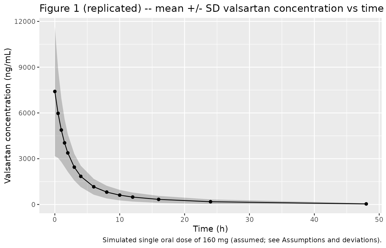
Simulated mean valsartan concentration vs time across the virtual cohort, plotted at the Kim 2015 nominal sampling times. The shaded ribbon shows mean +/- SD. Reproduces the format of Kim 2015 Figure 1.
Typical-subject profile
sim_typical |>
  filter(id == 1) |>
  ggplot(aes(time, Cc)) +
  geom_line(linewidth = 0.8) +
  scale_y_log10() +
  labs(x = "Time (h)",
       y = "Valsartan concentration (ng/mL, log10)",
       title = "Typical-subject profile after a 160 mg single oral dose")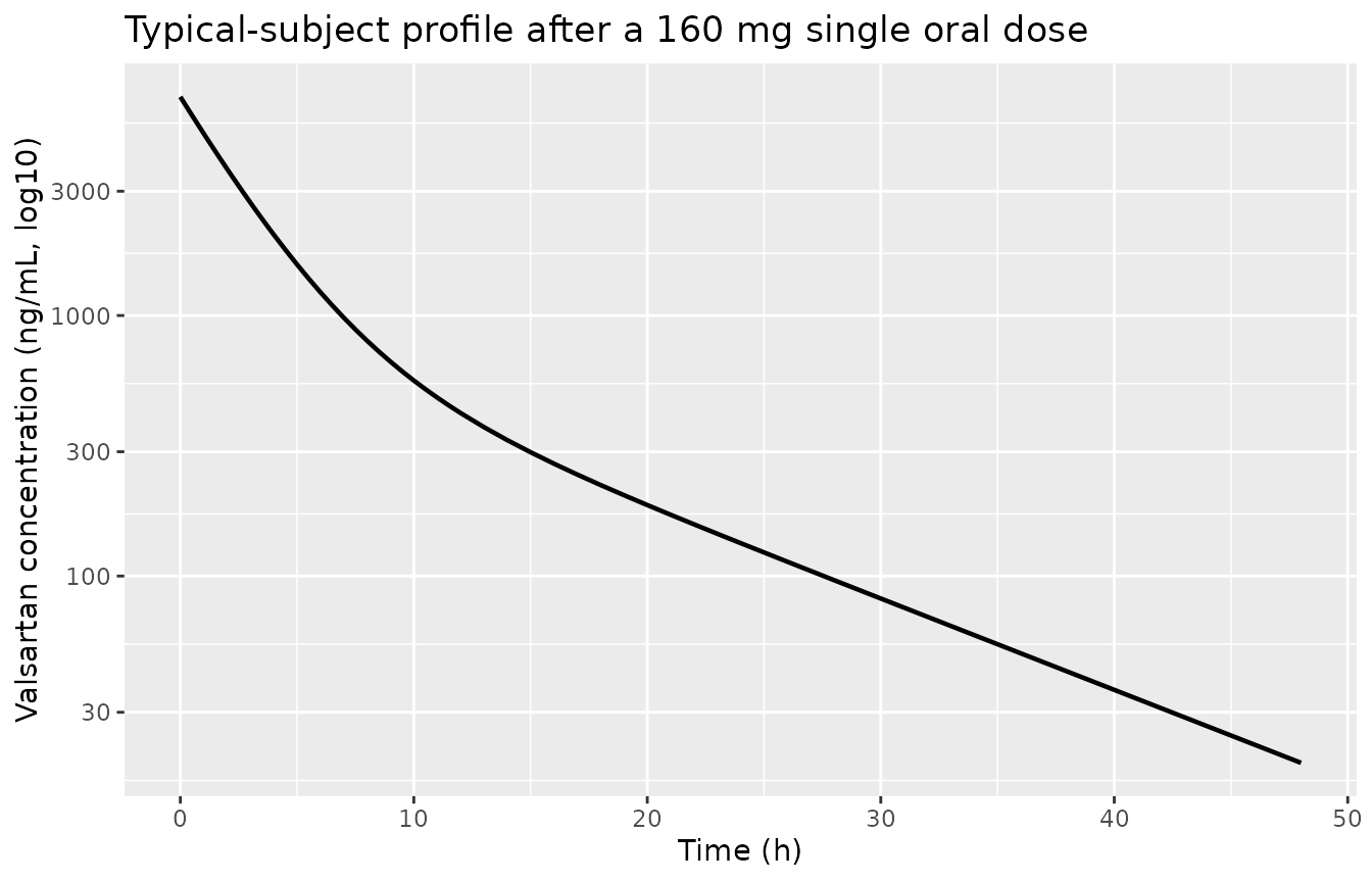
Simulated typical-subject (no IIV) valsartan concentration profile after a single 160 mg oral dose, plotted on a log-linear y axis to show both absorption and terminal-decay phases.
PKNCA validation
A standard single-dose NCA over the 0-48 h sampling window gives Cmax, Tmax, AUC0-inf, and half-life. Kim 2015 does not tabulate NCA values; the comparison below is internal to the simulation (cohort summary) and serves to confirm that the packaged model produces sensible single-dose PK characteristics for a 2-compartment zero-order-absorption parameterization at the reported parameter values.
nca_window <- sim |>
  filter(!is.na(Cc), time <= 48) |>
  select(id, time, Cc, cohort)

dose_df <- demo |>
  mutate(time = 0, amt = dose_mg) |>
  select(id, time, amt, cohort)

conc_obj <- PKNCA::PKNCAconc(nca_window, Cc ~ time | cohort + id)
dose_obj <- PKNCA::PKNCAdose(dose_df,    amt ~ time | cohort + id)

intervals <- data.frame(
  start      = 0,
  end        = Inf,
  cmax       = TRUE,
  tmax       = TRUE,
  aucinf.obs = TRUE,
  half.life  = TRUE
)

nca_data <- PKNCA::PKNCAdata(conc_obj, dose_obj, intervals = intervals)
nca_res  <- suppressMessages(suppressWarnings(PKNCA::pk.nca(nca_data)))
nca_summary <- summary(nca_res)
knitr::kable(
  nca_summary,
  caption = "Simulated single-dose NCA across the virtual cohort (160 mg oral)."
)| start | end | cohort | N | cmax | tmax | half.life | aucinf.obs |
|---|---|---|---|---|---|---|---|
| 0 | Inf | 160 mg single oral dose | 240 | 6370 [59.9] | 0.000 [0.000, 0.000] | 9.16 [1.60] | 26300 [43.3] |
Assumptions and deviations
Residual error not reported in Kim 2015. The paper describes a NONMEM SSE (stochastic simulation and estimation) workflow that necessarily defines
$SIGMA, but the numeric value is omitted from the publication and no supplement is available.propSdis approximated at 0.2 (20% proportional CV), a plausible default for a healthy-volunteer Phase I small-molecule oral popPK fit. The approximation does not load-bear the structural model or the CLCR-covariate effect that the paper is actually about; it only governs the spread of stochastic VPC ribbons. A downstream user who needs the published residual-error value should consult the corresponding author (K. S. Park, kspark@yuhs.ac).Dose magnitude not reported in Kim 2015. Kim 2015 Methods describes the sampling design (14 samples per subject, 0-48 h) but does not state the valsartan dose level used in the underlying study. The dose comes from the upstream Kim et al. 2013 fixed-dose-combination bioequivalence paper (Clin Ther 35:934-940), which is not on disk for this extraction. The vignette assumes a single 160 mg oral dose (the standard adult valsartan strength in the Korean Diovan / amlodipine-valsartan FDC product line). The model itself is dose-linear except for absorption duration; users can scale all simulated concentrations linearly by
actual_dose / 160if a different strength applies.Apparent oral parameters. All clearance and volume terms in the model are
CL/F,V1/F,Q/F,V2/F– bioavailabilityFis folded into the parameters and is not estimated separately. The model is therefore appropriate for oral dosing only; it cannot be used to predict IV exposure without re-introducingFfrom an independent source.CRCL is raw Cockcroft-Gault. Kim 2015 Table 1 reports CRCL in raw mL/min, not BSA-normalized to mL/min/1.73 m^2. The covariate column is stored as the canonical
CRCLperinst/references/covariate-columns.md, with the per-modelcovariateDataentry documenting the raw-mL/min units explicitly so the assay form is unambiguous to downstream users.Allometric exponents fixed. Kim 2015 Eq. 1 reports the exponents on CL/Q as the literal value 0.75 and on V1/V2 as 1.0 (linear
WT/70) with no uncertainty. These are encoded asfixed(0.75)andfixed(1)per the skill’s “fixed parameters” guidance.Power-experiment alternative THETA(6) values not encoded. Kim 2015 reports three values of
THETA(6)(0.793, 1.12, 1.19) corresponding to three significance levels in the power experiment. The estimated value is 0.793 (P = 0.0048); 1.12 and 1.19 were manually imposed by the authors for the simulation experiment, not alternative parameter estimates. The model encodes only the estimated 0.793 value.