Iruplinalkib translational dose selection (Yang 2025b)
Source:vignettes/articles/Yang_2025b_iruplinalkib.Rmd
Yang_2025b_iruplinalkib.RmdModel and source
- Citation: Yang G, Wang Y, Zhao H, Zheng Q, Wang X, Jia L, Xin Q, Ma C, Zhang Y, Zheng S, Kang X. Translational Model-Informed Dose Selection for Iruplinalkib, a Selective Oral ALK/ROS1 Tyrosine Kinase Inhibitor. Clin Transl Sci. 2025;18(7):e70287. doi:10.1111/cts.70287
- Article: https://doi.org/10.1111/cts.70287
- Full text and supplement (Methods S1, Figures S1-S3, Tables S1-S2): https://europepmc.org/article/PMC/PMC12254954
Iruplinalkib (WX-0593) is a selective oral ALK/ROS1 tyrosine kinase
inhibitor. Yang 2025 (Clin Transl Sci e70287; called “Yang 2025b” here
to separate it from the same group’s four-study population PK analysis,
Yang_2025_iruplinalkib) describes how the recommended phase
2 dose of 180 mg once daily was chosen. It combines three model layers,
each packaged as its own model file:
| Model | Layer | Fitted to |
|---|---|---|
Yang_2025b_iruplinalkib_mouse_ros1 |
Mouse PK + modified Simeoni tumor growth inhibition | ROS1-positive xenografts |
Yang_2025b_iruplinalkib_mouse_alk |
Same structure, ALK-specific tumor parameters | ALK-positive xenografts |
Yang_2025b_iruplinalkib_human |
Human PK projected from animal data | No human data (Wajima scaling) |
Yang_2025b_iruplinalkib |
Clinical population PK | WX-0593-001 patients + WX-0593-002 healthy volunteers |
The mouse tumor models give a tumor static concentration (TSC), which is converted to a human TSC through plasma protein binding. Each human PK model is then used to find the dose whose steady-state trough clears that TSC.
#> ℹ parameter labels from comments will be replaced by 'label()'| Model | Description |
|---|---|
| Yang_2025b_iruplinalkib_mouse_ros1 | Preclinical (mouse; female BALB/c-nu bearing subcutaneous SLC34A2-ROS1 Ba/F3 cell-line-derived xenografts). Iruplinalkib PK-PD tumor growth inhibition model: a two-compartment PK model with first-order oral absorption, fitted first to the plasma data of the same mice and then held fixed, drives a modified Simeoni model in which exponential-then- linear tumor growth (switch sharpness psi = 20) is opposed by an Emax kill of proliferating cells (Kmax, KC50) followed by three damaged-cell transit compartments. Typical-value model. |
| Yang_2025b_iruplinalkib_mouse_alk | Preclinical (mouse; female BALB/c-nu bearing subcutaneous ALK-addicted NCI-H3122 cell-line-derived xenografts). Iruplinalkib PK-PD tumor growth inhibition model: a two-compartment PK model with first-order oral absorption, fitted to plasma data from the companion ROS1-xenograft mice and held fixed (no PK was sampled in the ALK-xenograft mice), drives a modified Simeoni model in which exponential-then- linear tumor growth (switch sharpness psi = 20) is opposed by an Emax kill of proliferating cells (Kmax, KC50) followed by three damaged-cell transit compartments. Typical-value model. |
| Yang_2025b_iruplinalkib_human | Animal-scaled human projection (not fitted to human data). Two-compartment PK model with first-order absorption and first-order elimination for oral iruplinalkib (WX-0593, a selective ALK/ROS1 tyrosine kinase inhibitor), built before the first clinical data were available to predict the human effective dose. Mouse, rat, dog and monkey intravenous profiles were superimposed with Wajima’s Css-MRT normalisation and rescaled to a 60 kg human using predicted Vss (7.9 L/kg) and CL (311 mL/min) averaged over several interspecies methods; a two-compartment model was fitted to the rescaled profile and combined with the mean animal oral bioavailability (59.2%) and the monkey Ka (0.341 1/h) to give apparent oral parameters. Typical-value model with no variability. |
| Yang_2025b_iruplinalkib | Two-compartment population PK model with first-order absorption and first-order elimination for oral iruplinalkib (WX-0593, a selective ALK/ROS1 tyrosine kinase inhibitor), fitted to the early clinical data used to select the recommended phase 2 dose: the phase 1 dose-escalation and expansion trial WX-0593-001 in patients with ALK- or ROS1-positive advanced non-small-cell lung cancer and the single-dose 120 mg food-effect study WX-0593-002 in healthy volunteers. Apparent oral clearance carries power effects of baseline body weight and serum albumin, and the apparent central volume a power effect of baseline body weight. Dosing in the fed state multiplies the absorption rate constant by 0.796 and adds a 0.479 h absorption lag. Residual error is proportional, with a separate magnitude for each of the two studies. |
Population
Mouse. Female BALB/c-nu mice were implanted subcutaneously with SLC34A2-ROS1-overexpressing Ba/F3 cells or ALK-addicted NCI-H3122 cells. Once tumors reached 100-300 mm^3 the mice (n = 9 per group) received oral iruplinalkib once daily: 0, 5, 10 or 20 mg/kg for 14 days (ROS1) or 0, 2.5, 5 or 10 mg/kg for 21 days (ALK). Plasma was sampled before dosing and 1, 2, 4, 8 and 24 h after the final Day-14 dose in the ROS1 mice only (Methods “Mouse Xenograft Study” and “Mouse PKPD Modeling”).
Human projection. No subjects. Mouse, rat, dog and monkey PK were scaled to a 60 kg human (Methods “Prediction of Human PK Parameters” and Methods S1).
Clinical. The PopPK dataset pooled the first-in-human dose-escalation and expansion trial WX-0593-001 in Chinese patients with ALK- or ROS1-positive advanced non-small-cell lung cancer and the healthy-volunteer food-effect study WX-0593-002 (a single 120 mg dose). The paper prints no demographic table and does not give the number of subjects in the dataset. The steady-state simulations used the 54 WX-0593-001 patients dosed at 120, 180 or 240 mg once daily.
The same information is available programmatically via, e.g.,
readModelDb("Yang_2025b_iruplinalkib")()$population.
Source trace
All four files carry an in-file comment naming the source of every
ini() value. They are collected here.
| Model | Parameter | Value | Source |
|---|---|---|---|
| mouse (both) |
lka, lcl, lvc,
lq, lvp
|
0.366 1/h, 2.48 L/h/kg, 3.59 L/kg, 0.0843 L/h/kg, 1.65 L/kg (all
fixed) |
Table S1 |
| mouse (both) | propSd |
0.46 (fixed) |
Table S1 proportional residual 46% |
| mouse ROS1 |
ltumorExpGrowth, ltumorLinGrowth
|
0.00851 1/h, 4.45 mm^3/h | Table 1, ROS1 column (lambda0, lambda1) |
| mouse ROS1 |
lkmax, lkc50
|
0.0739 1/h, 1221 ng/mL | Table 1, ROS1 column |
| mouse ROS1 |
ldamageTransit, lrbase_tumor
|
0.168 1/h, 221 mm^3 | Table 1, ROS1 column (K1, E0) |
| mouse ALK |
ltumorExpGrowth, ltumorLinGrowth
|
0.006515 1/h, 3.17 mm^3/h | Table 1, ALK column |
| mouse ALK |
lkmax, lkc50
|
0.092 1/h, 1674 ng/mL | Table 1, ALK column |
| mouse ALK |
ldamageTransit, lrbase_tumor
|
0.0524 1/h, 200 mm^3 | Table 1, ALK column |
| mouse (both) | psi |
20 (fixed) |
Table 1 (FIX) |
| mouse (both) | propSd_tumor_vol |
0 (fixed) |
Not reported |
| mouse (both) | tumor ODEs | n/a | Methods S1 Eq1-7; Figure 1B |
| human projection | lka |
0.341 1/h (fixed) |
Table 2 (FIX); Methods S1 monkey Ka |
| human projection |
lcl, lvc, lq,
lvp
|
33.7 L/h, 379 L, 134 L/h, 239 L | Table 2 |
| clinical |
lka, lcl, lvc,
lq, lvp
|
1.11 1/h, 20.5 L/h, 342 L, 14.8 L/h, 336 L | Table 3 |
| clinical | ltlag |
0.479 h (fed only) | Table 3 ‘ALAG for fed subjects’ |
| clinical | e_fed_ka |
0.796 | Table 3 ‘Food on Ka’ |
| clinical |
e_alb_cl, e_wt_base_cl,
e_wt_base_vc
|
1.23, 0.713, 2.02 | Table 3; footnote equations (ALB/42), (BBWT/63) |
| clinical |
etalka, etalcl, etalvc
|
0.513, 0.0940, 0.163 | Table 3 IIV 81.9%, 31.4%, 42.1%; omega^2 = log(1 + CV^2) |
| clinical |
propSdPatient, propSdHv
|
0.326, 0.547 | Table 3 residual errors for WX-0593-001 and -002 |
The modified Simeoni model of Methods S1 is
with three transit compartments at rate
carrying damaged cells to death
(
= cycling_cells,
-
= damaged_cells1-damaged_cells3).
is the plasma concentration in ng/mL, and
.
Mouse PK (Figure S1A)
The mouse PK parameters were fitted once to the ROS1-xenograft plasma data and then held fixed in both tumor fits. Both mouse files carry the same PK. The paper gives no between-animal variability for either stage, so these are typical-value simulations.
# Observation rows nominate an endpoint through dvid (1 = Cc, 2 = tumor_vol);
# cmt stays NA on observation rows, so no observable is used as a compartment.
mouse_events <- function(dose, n_doses, obs_times, dvid = 1L) {
  dplyr::bind_rows(
    data.frame(
      time = (seq_len(n_doses) - 1) * 24, amt = dose, cmt = "depot",
      evid = 1L, dvid = NA_integer_
    ),
    data.frame(
      time = obs_times, amt = NA_real_, cmt = NA_character_,
      evid = 0L, dvid = dvid
    )
  ) |>
    dplyr::arrange(time, dplyr::desc(evid))
}

# The mouse models carry no etas, so a plain solve is the typical-value
# prediction (Cc and tumor_vol are the noise-free predictions).
solve_typical <- function(mod, events) {
  as.data.frame(rxode2::rxSolve(mod, events, returnType = "data.frame"))
}

mod_ros1 <- readModelDb("Yang_2025b_iruplinalkib_mouse_ros1")
mod_alk <- readModelDb("Yang_2025b_iruplinalkib_mouse_alk")
last_dose <- 13 * 24
pk_grid <- last_dose + c(seq(0, 2, by = 0.1), seq(2.25, 24, by = 0.25))

mouse_pk <- lapply(c(5, 10, 20), function(d) {
  solve_typical(mod_ros1, mouse_events(d, 14, pk_grid)) |>
    dplyr::mutate(dose = d, tad = time - last_dose)
}) |>
  dplyr::bind_rows()

# Group means read off Figure S1A by the maintainers (ng/mL); the paper does
# not tabulate them.
s1a <- tibble::tribble(
  ~dose, ~tad, ~Cc,
  5, 2, 390, 5, 4, 195, 5, 8, 55,
  10, 2, 1230, 10, 4, 520, 10, 8, 170,
  20, 2, 1450, 20, 4, 830, 20, 8, 490
)

ggplot(mouse_pk, aes(tad, Cc, colour = factor(dose))) +
  geom_line() +
  geom_point(data = s1a, shape = 1, size = 2.5) +
  labs(
    x = "Time after the Day-14 dose (h)", y = "Iruplinalkib (ng/mL)",
    colour = "Dose (mg/kg)",
    caption = "Lines: typical-value model. Circles: Figure S1A group means (digitised)."
  )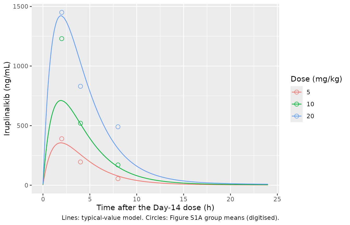
The model sits on the observed means at 5 and 20 mg/kg (2 h peaks 355 vs 390 and 1421 vs 1450 ng/mL). At 10 mg/kg the observed peak (about 1230 ng/mL) is close to the 20 mg/kg peak, so exposure in these mice was not dose-proportional. A linear model fitted to all three doses cannot follow that, and it under-predicts the 10 mg/kg group.
A PKNCA check of the steady-state interval confirms the disposition: for a linear model at steady state, AUC over one dosing interval equals dose / (CL/F).
mouse_nca_in <- mouse_pk |>
  dplyr::filter(!is.na(Cc)) |>
  dplyr::mutate(treatment = paste(dose, "mg/kg"), time = tad, id = 1L) |>
  dplyr::select(id, treatment, time, Cc)
mouse_dose <- mouse_nca_in |>
  dplyr::distinct(id, treatment) |>
  dplyr::mutate(time = 0, amt = as.numeric(sub(" mg/kg", "", treatment)))

mouse_nca <- PKNCA::pk.nca(PKNCA::PKNCAdata(
  PKNCA::PKNCAconc(mouse_nca_in, Cc ~ time | treatment + id),
  PKNCA::PKNCAdose(mouse_dose, amt ~ time | treatment + id),
  intervals = data.frame(start = 0, end = 24, cmax = TRUE, tmax = TRUE, auclast = TRUE),
  options = list(auc.method = "linear")
))

mouse_auc <- as.data.frame(mouse_nca$result) |>
  dplyr::filter(PPTESTCD == "auclast") |>
  dplyr::mutate(
    dose = as.numeric(sub(" mg/kg", "", treatment)),
    expected = dose / 2.48 * 1000,
    pct_diff = 100 * (PPORRES - expected) / expected
  )
mouse_auc |>
  dplyr::select(treatment, PPORRES, expected, pct_diff) |>
  dplyr::rename(
    "Dose" = treatment, "Simulated AUC0-24 (ng*h/mL)" = PPORRES,
    "Dose / (CL/F) (ng*h/mL)" = expected, "% difference" = pct_diff
  ) |>
knitr::kable(digits = 1)| Dose | Simulated AUC0-24 (ng*h/mL) | Dose / (CL/F) (ng*h/mL) | % difference |
|---|---|---|---|
| 10 mg/kg | 4031.5 | 4032.3 | 0 |
| 20 mg/kg | 8062.9 | 8064.5 | 0 |
| 5 mg/kg | 2015.7 | 2016.1 | 0 |
Mouse tumor growth inhibition (Figures S1B, S1C)
tgi_sim <- function(mod, doses, n_doses) {
  t_end <- n_doses * 24
  lapply(doses, function(d) {
    solve_typical(mod, mouse_events(d, n_doses, seq(0, t_end, by = 2), dvid = 2L)) |>
      dplyr::mutate(dose = d)
  }) |>
    dplyr::bind_rows()
}

tgi_ros1 <- tgi_sim(mod_ros1, c(0, 5, 10, 20), 14) |> dplyr::mutate(model = "ROS1")
tgi_alk <- tgi_sim(mod_alk, c(0, 2.5, 5, 10), 21) |> dplyr::mutate(model = "ALK")
tgi <- dplyr::bind_rows(tgi_ros1, tgi_alk)

# Group means read off Figures S1B and S1C by the maintainers (mm^3). Day 1 is
# the first dose, i.e. model time 0.
s1bc <- dplyr::bind_rows(
  tibble::tibble(
    model = "ROS1", day = rep(c(1, 5, 8, 12, 15), 4),
    dose = rep(c(0, 5, 10, 20), each = 5),
    tumor_vol = c(
      230, 500, 740, 1280, 1600,
      230, 440, 630, 860, 970,
      230, 280, 380, 530, 540,
      230, 140, 230, 270, 270
    )
  ),
  tibble::tibble(
    model = "ALK", day = rep(c(1, 4, 7, 10, 14, 17, 21), 4),
    dose = rep(c(0, 2.5, 5, 10), each = 7),
    tumor_vol = c(
      180, 330, 500, 780, 1010, 1220, 1600,
      180, 290, 450, 600, 690, 890, 975,
      180, 260, 370, 430, 530, 620, 730,
      180, 200, 200, 230, 240, 220, 230
    )
  )
) |>
  dplyr::mutate(time = (day - 1) * 24)

ggplot(tgi, aes(time / 24 + 1, tumor_vol, colour = factor(dose))) +
  geom_line() +
  geom_point(data = s1bc, shape = 1, size = 2.5) +
  facet_wrap(~model, scales = "free_x") +
  labs(
    x = "Study day", y = "Tumor volume (mm^3)", colour = "Dose (mg/kg)",
    caption = "Lines: typical-value model. Circles: Figures S1B/S1C group means (digitised)."
  )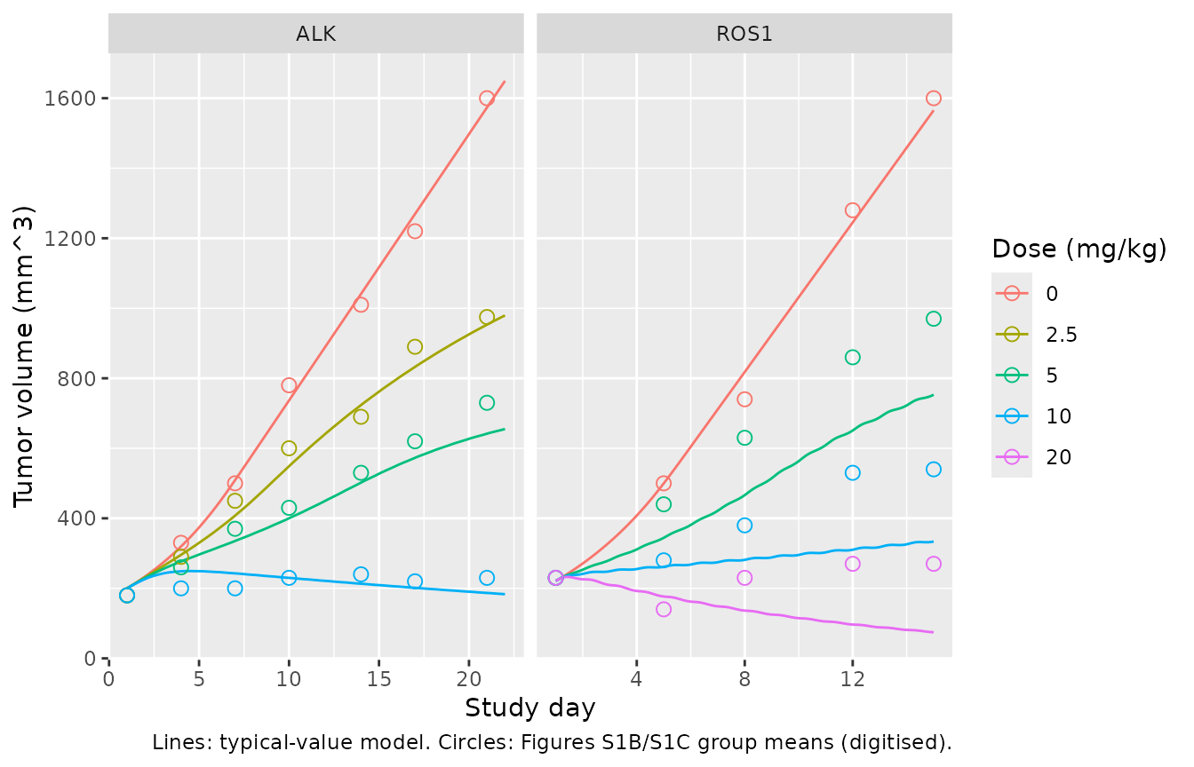
The paper reports the tumor growth inhibition (TGI) range for each xenograft (46.1-97.1% ROS1, 44.1-95.8% ALK, Results) but not its formula. The usual definition, 1 - (change in treated volume) / (change in control volume) at the end of treatment, gives 46%, 97%, 44% and 96% from the digitised Figure S1 means. That agreement supports reading the reported values with this definition.
tgi_end <- tgi |>
  dplyr::group_by(model) |>
  dplyr::filter(time == max(time)) |>
  dplyr::mutate(
    v0 = ifelse(model == "ROS1", 221, 200),
    ctrl = tumor_vol[dose == 0],
    TGI = 100 * (1 - (tumor_vol - v0) / (ctrl - v0))
  ) |>
  dplyr::ungroup()

tgi_ref <- tibble::tribble(
  ~model, ~dose, ~TGI_paper,
  "ROS1", 5, 46.1, "ROS1", 20, 97.1,
  "ALK", 2.5, 44.1, "ALK", 10, 95.8
)
tgi_cmp <- tgi_end |>
  dplyr::filter(dose > 0) |>
  dplyr::left_join(tgi_ref, by = c("model", "dose")) |>
  dplyr::select(model, dose, tumor_vol, TGI, TGI_paper)
tgi_cmp |>
  dplyr::rename(
    "Xenograft" = model, "Dose (mg/kg)" = dose,
    "Simulated end volume (mm^3)" = tumor_vol, "Simulated TGI (%)" = TGI,
    "Reported TGI (%)" = TGI_paper
  ) |>
knitr::kable(digits = 1)| Xenograft | Dose (mg/kg) | Simulated end volume (mm^3) | Simulated TGI (%) | Reported TGI (%) |
|---|---|---|---|---|
| ROS1 | 5.0 | 753.1 | 60.4 | 46.1 |
| ROS1 | 10.0 | 333.8 | 91.6 | NA |
| ROS1 | 20.0 | 74.5 | 110.9 | 97.1 |
| ALK | 2.5 | 979.6 | 46.2 | 44.1 |
| ALK | 5.0 | 655.1 | 68.6 | NA |
| ALK | 10.0 | 183.4 | 101.1 | 95.8 |
ctrl_end <- tgi_end |> dplyr::filter(dose == 0)
stopifnot(
  # Untreated growth: lambda0, lambda1, psi and E0 alone reproduce the control
  # arm (digitised end volume about 1600 mm^3 in both xenografts).
  all(abs(ctrl_end$tumor_vol / 1600 - 1) < 0.10),
  # Typical-value model, deterministic: realised gaps are 14.3, 13.8, 2.1 and
  # 5.3 percentage points. A mis-transcribed Kmax or KC50 moves these by tens
  # of points.
  all(abs(tgi_cmp$TGI[!is.na(tgi_cmp$TGI_paper)] - tgi_cmp$TGI_paper[!is.na(tgi_cmp$TGI_paper)]) < 20)
)
The ALK model matches the reported TGI within about 5 points at both ends of the dose range (46 vs 44% at 2.5 mg/kg, 101 vs 96% at 10 mg/kg). The ROS1 model gives more inhibition than the observed means at every dose (60 vs 46% at 5 mg/kg). At 20 mg/kg it shrinks the tumor (TGI above 100%), whereas the observed mean shrank to about 140 mm^3 by Day 5 and then grew back to about 270 mm^3. A Simeoni model with linear PK cannot regrow under constant dosing. The gap is plausibly the difference between a typical-value curve and a mean of animals: the fit was population-based (FOCE-ELS), but its between-animal variability is not reported, so the mean prediction cannot be rebuilt.
Tumor static concentration
At the tumor static concentration, kill balances exponential-phase growth: TSC = lambda0 * KC50 / (Kmax - lambda0). The human TSC rescales it by the unbound fraction, mouse 15% (85% bound) and human 24.3% (75.7% bound; Results and Discussion).
tsc_tab <- lapply(list(ROS1 = mod_ros1, ALK = mod_alk), function(m) {
  ini <- rxode2::rxode(m)$theta
  l0 <- exp(ini[["ltumorExpGrowth"]])
  kc50 <- exp(ini[["lkc50"]])
  kmax <- exp(ini[["lkmax"]])
  tsc <- l0 * kc50 / (kmax - l0)
  data.frame(tsc_mouse = tsc, tsc_human = tsc * 0.15 / 0.243)
}) |>
  dplyr::bind_rows(.id = "model") |>
  dplyr::mutate(
    tsc_mouse_paper = c(159, 127),
    tsc_human_paper = c(98, 78)
  ) |>
  dplyr::relocate(tsc_mouse_paper, .after = tsc_mouse)
tsc_tab |>
  dplyr::rename(
    "Xenograft" = model, "Mouse TSC (ng/mL)" = tsc_mouse,
    "Paper mouse TSC" = tsc_mouse_paper, "Human TSC (ng/mL)" = tsc_human,
    "Paper human TSC" = tsc_human_paper
  ) |>
knitr::kable(digits = 1)| Xenograft | Mouse TSC (ng/mL) | Paper mouse TSC | Human TSC (ng/mL) | Paper human TSC |
|---|---|---|---|---|
| ROS1 | 158.9 | 159 | 98.1 | 98 |
| ALK | 127.6 | 127 | 78.8 | 78 |
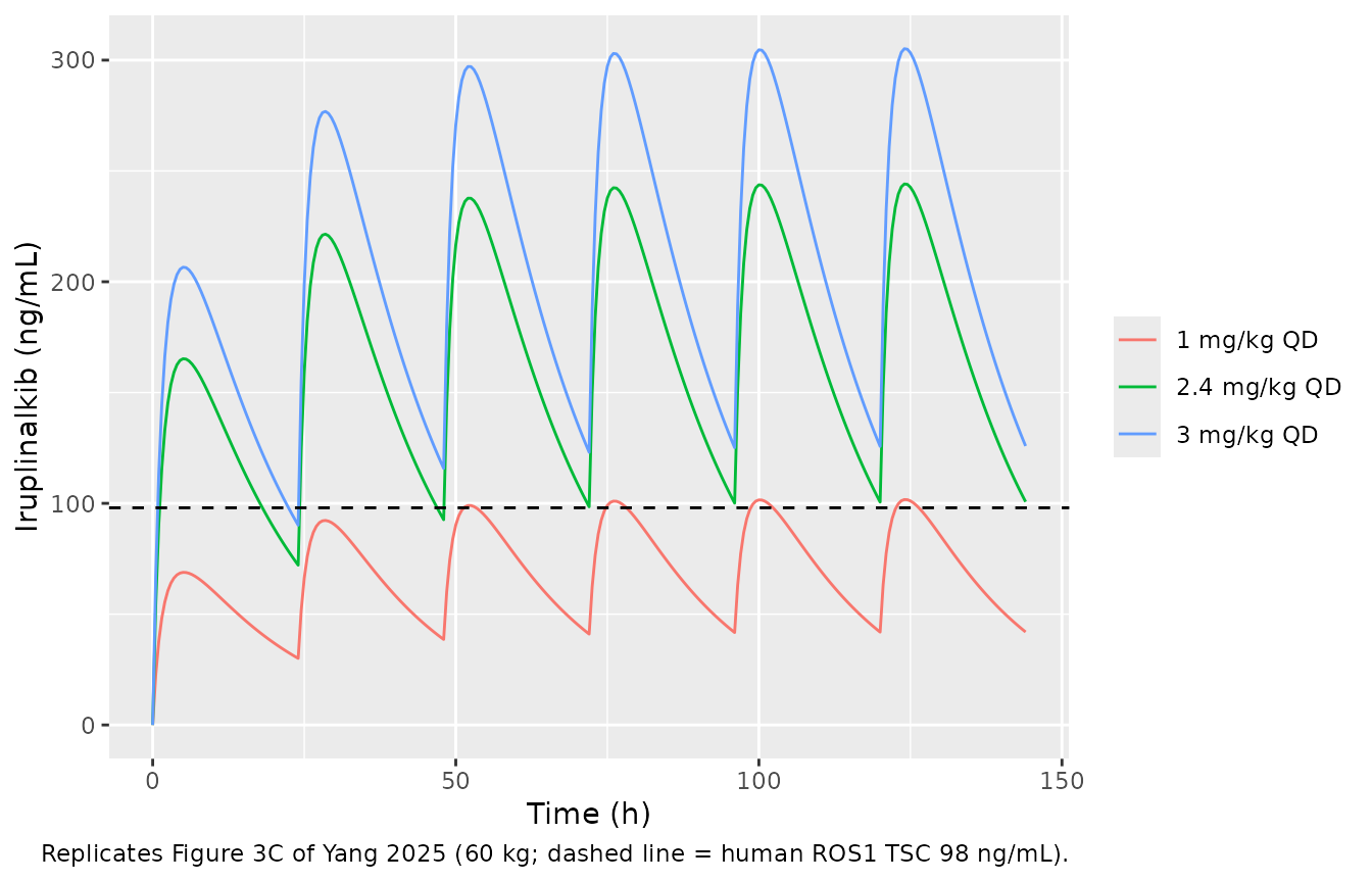
Human PK projected from animals (Figure 3C, Table S2)
Table 2 labels its parameters as apparent oral values (CL/F, V1/F, Q/F, V2/F), so the model applies no separate bioavailability. Two checks show the 59.2% is already divided in. Simulating 180 mg once daily reproduces the paper’s preclinical projection in Table S2 exactly. And the earliest points of the 1 mg/kg (60 mg) intravenous profile in Figure 3B, about 200-330 ng/mL, bracket dose / V1 = 268 ng/mL for V1 = 379 x 0.592 = 224 L; V1 = 379 L would give 158 ng/mL.
mod_hp <- readModelDb("Yang_2025b_iruplinalkib_human")
hp_events <- function(dose_mg, n_doses = 30, obs = seq(0, n_doses * 24, by = 0.25)) {
  rxode2::et(amt = dose_mg, ii = 24, addl = n_doses - 1, cmt = "depot") |>
    rxode2::et(obs, cmt = "central")
}

fig3c <- lapply(c(1, 2.4, 3), function(mgkg) {
  as.data.frame(rxode2::rxSolve(mod_hp, hp_events(mgkg * 60, 6, seq(0, 144, by = 0.5)))) |>
    dplyr::mutate(regimen = paste(mgkg, "mg/kg QD"))
}) |>
  dplyr::bind_rows()

ggplot(fig3c, aes(time, Cc * 1000, colour = regimen)) +
  geom_line() +
  geom_hline(yintercept = 98, linetype = "dashed") +
  labs(
    x = "Time (h)", y = "Iruplinalkib (ng/mL)", colour = NULL,
    caption = "Replicates Figure 3C of Yang 2025 (60 kg; dashed line = human ROS1 TSC 98 ng/mL)."
  )
hp_ss <- as.data.frame(rxode2::rxSolve(mod_hp, hp_events(180))) |>
  dplyr::filter(time >= 29 * 24)
hp_cmp <- tibble::tibble(
  quantity = c("Ctrough,ss", "Cmax,ss"),
  simulated = c(1000 * hp_ss$Cc[hp_ss$time == 30 * 24], 1000 * max(hp_ss$Cc)),
  table_s2 = c(126, 305)
)
knitr::kable(
  hp_cmp |> dplyr::rename(
    "180 mg QD" = quantity, "Simulated (ng/mL)" = simulated,
    "Table S2 preclinical (ng/mL)" = table_s2
  ),
  digits = 1
)| 180 mg QD | Simulated (ng/mL) | Table S2 preclinical (ng/mL) |
|---|---|---|
| Ctrough,ss | 125.9 | 126 |
| Cmax,ss | 305.4 | 305 |
The paper’s projected effective dose, 2.4 mg/kg (144 mg) once daily, gives a steady-state trough just above the 98 ng/mL ROS1 TSC, as in Figure 3C.
Clinical population PK (Figure 4, Table S2)
Food effect
Food slows absorption (Ka x 0.796, plus a 0.479 h lag) but leaves CL/F unchanged. So a fed dose must give the same AUC as a fasted one, equal to dose / (CL/F) for the reference subject.
mod_clin <- readModelDb("Yang_2025b_iruplinalkib")
food_ev <- dplyr::bind_rows(
  data.frame(id = 1L, time = 0, amt = 120, cmt = "depot", evid = 1L, FED = 0),
  data.frame(id = 1L, time = c(seq(0, 12, by = 0.05), seq(12.5, 480, by = 0.5)), amt = NA, cmt = "central", evid = 0L, FED = 0),
  data.frame(id = 2L, time = 0, amt = 120, cmt = "depot", evid = 1L, FED = 1),
  data.frame(id = 2L, time = c(seq(0, 12, by = 0.05), seq(12.5, 480, by = 0.5)), amt = NA, cmt = "central", evid = 0L, FED = 1)
) |>
  dplyr::mutate(WT_BASE = 63, ALB = 42, STUDY_WX0593_002 = 1) |>
  dplyr::arrange(id, time, dplyr::desc(evid))

# zeroRe() warns that the typical-value model has no omega or sigma left;
# that is the intent here.
food_sim <- suppressWarnings(
  as.data.frame(rxode2::rxSolve(rxode2::zeroRe(mod_clin), food_ev, keep = "FED"))
)
#> ℹ parameter labels from comments will be replaced by 'label()'
#> ℹ omega/sigma items treated as zero: 'etalka', 'etalcl', 'etalvc'
ggplot(dplyr::filter(food_sim, time <= 24), aes(time, Cc * 1000, colour = factor(FED, labels = c("Fasted", "Fed")))) +
  geom_line() +
  labs(x = "Time after a single 120 mg dose (h)", y = "Iruplinalkib (ng/mL)", colour = NULL)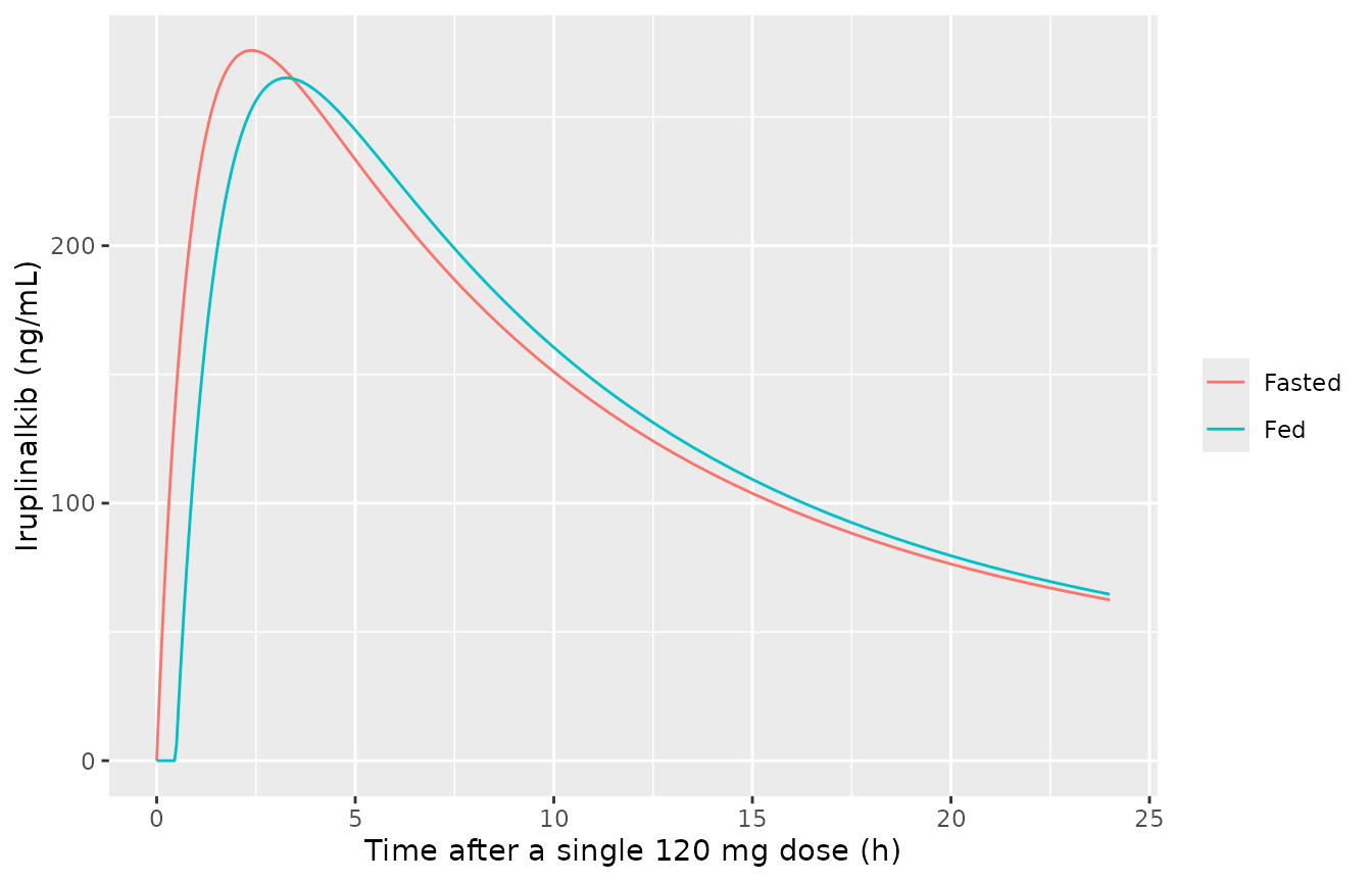
food_nca_in <- food_sim |>
  dplyr::filter(!is.na(Cc)) |>
  dplyr::mutate(treatment = ifelse(FED == 1, "Fed", "Fasted"), Cc = Cc * 1000) |>
  dplyr::select(id, treatment, time, Cc)
food_nca <- PKNCA::pk.nca(PKNCA::PKNCAdata(
  PKNCA::PKNCAconc(food_nca_in, Cc ~ time | treatment + id),
  PKNCA::PKNCAdose(
    food_nca_in |> dplyr::distinct(id, treatment) |> dplyr::mutate(time = 0, amt = 120),
    amt ~ time | treatment + id
  ),
  intervals = data.frame(start = 0, end = Inf, cmax = TRUE, tmax = TRUE, aucinf.obs = TRUE, half.life = TRUE)
))
food_res <- as.data.frame(food_nca$result) |>
  dplyr::filter(PPTESTCD %in% c("cmax", "tmax", "aucinf.obs")) |>
  dplyr::select(treatment, PPTESTCD, PPORRES) |>
  tidyr::pivot_wider(names_from = PPTESTCD, values_from = PPORRES)
food_res |>
  dplyr::rename(
    "State" = treatment, "Cmax (ng/mL)" = cmax, "Tmax (h)" = tmax,
    "AUC0-inf (ng*h/mL)" = aucinf.obs
  ) |>
knitr::kable(digits = 1)| State | Cmax (ng/mL) | Tmax (h) | AUC0-inf (ng*h/mL) |
|---|---|---|---|
| Fasted | 275.9 | 2.4 | 5853.7 |
| Fed | 265.2 | 3.2 | 5853.8 |
Steady-state exposure at 120, 180 and 240 mg once daily
The paper overlaid its simulations on the 54 WX-0593-001 patients but does not report their body weight or albumin. The virtual cohort below assumes body weight log-normal around the 63 kg reference (log-scale SD 0.16) and albumin normal around the 42 g/L reference (SD 4 g/L), both truncated to plausible adult ranges. All patients are dosed fasted and carry the WX-0593-001 residual error.
rxode2::rxSetSeed(20250707)
set.seed(20250707)
n_per_arm <- 200
doses <- c(120, 180, 240)

make_arm <- function(dose, id_offset) {
  subj <- tibble::tibble(
    id = id_offset + seq_len(n_per_arm),
    WT_BASE = pmin(pmax(exp(rnorm(n_per_arm, log(63), 0.16)), 40), 95),
    ALB = pmin(pmax(rnorm(n_per_arm, 42, 4), 28), 54),
    treatment = paste(dose, "mg QD")
  )
  dose_rows <- subj |>
    tidyr::crossing(time = seq(0, 20 * 24, by = 24)) |>
    dplyr::mutate(amt = dose, cmt = "depot", evid = 1L)
  obs_rows <- subj |>
    tidyr::crossing(time = 20 * 24 + c(seq(0, 4, by = 0.25), seq(4.5, 24, by = 0.5))) |>
    dplyr::mutate(amt = NA_real_, cmt = "central", evid = 0L)
  dplyr::bind_rows(dose_rows, obs_rows)
}

clin_events <- dplyr::bind_rows(lapply(seq_along(doses), function(i) {
  make_arm(doses[i], (i - 1) * n_per_arm)
})) |>
  dplyr::mutate(FED = 0, STUDY_WX0593_002 = 0) |>
  dplyr::arrange(id, time, dplyr::desc(evid))
stopifnot(!anyDuplicated(unique(clin_events[, c("id", "time", "evid")])))

clin_sim <- as.data.frame(rxode2::rxSolve(mod_clin, clin_events, keep = "treatment")) |>
  dplyr::mutate(Cc_ng = Cc * 1000, tad = time - 20 * 24)
#> ℹ parameter labels from comments will be replaced by 'label()'
clin_sim |>
  dplyr::group_by(treatment, tad) |>
  dplyr::summarise(
    Q05 = quantile(Cc_ng, 0.05), Q50 = median(Cc_ng), Q95 = quantile(Cc_ng, 0.95),
    .groups = "drop"
  ) |>
  ggplot(aes(tad, Q50, colour = treatment, fill = treatment)) +
  geom_ribbon(aes(ymin = Q05, ymax = Q95), alpha = 0.2, colour = NA) +
  geom_line(linewidth = 1) +
  scale_y_log10() +
  labs(
    x = "Time after dose at steady state (h)", y = "Iruplinalkib (ng/mL)",
    colour = NULL, fill = NULL,
    caption = "Replicates Figure 4 of Yang 2025: median and 90% prediction interval."
  )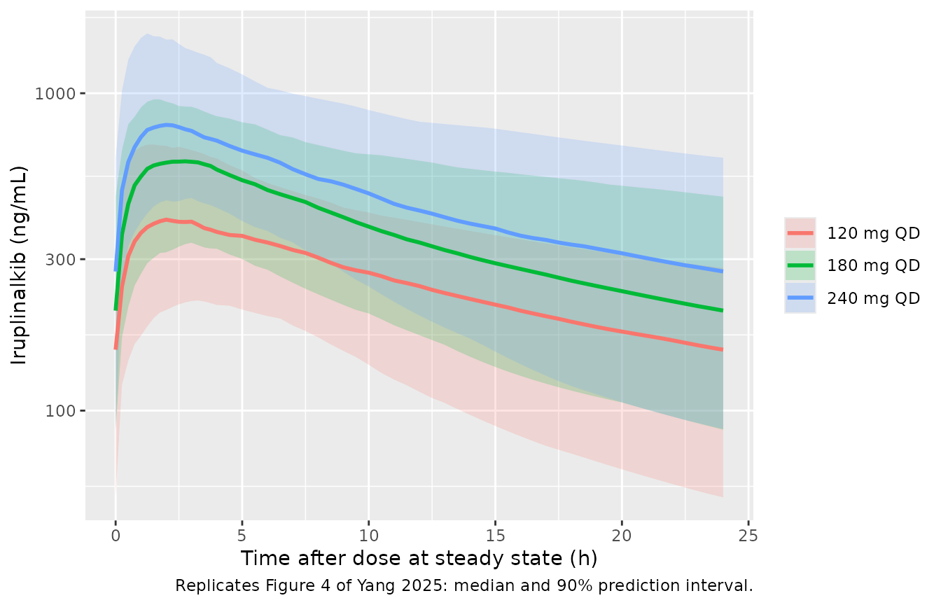
The paper states its steady-state troughs twice. The Results give the median (10th, 90th percentile) as 151 (71.4, 293), 232 (109, 449) and 301 (142, 588) ng/mL for 120, 180 and 240 mg. Table S2 gives a 180 mg median (5th-95th) of 210 (82-444) ng/mL for the trough and 635 (389-1024) ng/mL for Cmax. These are two simulations of the same model whose cohorts are not described.
clin_nca_in <- clin_sim |>
  dplyr::filter(!is.na(Cc_ng)) |>
  dplyr::transmute(id, treatment, time = tad, Cc = Cc_ng)
clin_dose <- clin_nca_in |>
  dplyr::distinct(id, treatment) |>
  dplyr::mutate(time = 0, amt = as.numeric(sub(" mg QD", "", treatment)))
clin_nca <- PKNCA::pk.nca(PKNCA::PKNCAdata(
  PKNCA::PKNCAconc(clin_nca_in, Cc ~ time | treatment + id),
  PKNCA::PKNCAdose(clin_dose, amt ~ time | treatment + id),
  intervals = data.frame(start = 0, end = 24, cmax = TRUE, cmin = TRUE, auclast = TRUE),
  options = list(auc.method = "linear")
))

# At steady state with no lag (fasted), the interval minimum is the trough.
clin_ind <- as.data.frame(clin_nca$result) |>
  dplyr::filter(PPTESTCD %in% c("cmin", "cmax")) |>
  dplyr::select(id, treatment, PPTESTCD, PPORRES) |>
  tidyr::pivot_wider(names_from = PPTESTCD, values_from = PPORRES)

clin_tab <- clin_ind |>
  dplyr::group_by(treatment) |>
  dplyr::summarise(
    trough_p10 = quantile(cmin, 0.10), trough_p50 = median(cmin),
    trough_p90 = quantile(cmin, 0.90),
    pct_above_tsc = 100 * mean(cmin > 98),
    .groups = "drop"
  ) |>
  dplyr::mutate(
    paper_p10 = c(71.4, 109, 142), paper_p50 = c(151, 232, 301),
    paper_p90 = c(293, 449, 588)
  )
clin_tab |>
  dplyr::rename(
    "Regimen" = treatment, "Sim P10" = trough_p10, "Sim median" = trough_p50,
    "Sim P90" = trough_p90, "Paper P10" = paper_p10, "Paper median" = paper_p50,
    "Paper P90" = paper_p90, "% above 98 ng/mL" = pct_above_tsc
  ) |>
  dplyr::relocate("Paper P10", .after = "Sim P10") |>
  dplyr::relocate("Paper median", .after = "Sim median") |>
  dplyr::relocate("Paper P90", .after = "Sim P90") |>
knitr::kable(digits = 1, caption = "Steady-state trough (ng/mL) vs Yang 2025 Results.")| Regimen | Sim P10 | Paper P10 | Sim median | Paper median | Sim P90 | Paper P90 | % above 98 ng/mL |
|---|---|---|---|---|---|---|---|
| 120 mg QD | 70.4 | 71.4 | 155.6 | 151 | 253.5 | 293 | 77.5 |
| 180 mg QD | 99.7 | 109.0 | 206.6 | 232 | 404.5 | 449 | 91.0 |
| 240 mg QD | 118.3 | 142.0 | 274.4 | 301 | 514.5 | 588 | 93.0 |
cmp <- nlmixr2lib::ncaComparisonTable(
  simulated = clin_nca,
  reference = tibble::tibble(treatment = "180 mg QD", cmax = 635, cmin = 210),
  by = "treatment",
  params = c("cmax", "cmin"),
  units = c(cmax = "ng/mL", cmin = "ng/mL"),
  tolerance_pct = 20
)
knitr::kable(cmp, caption = "180 mg QD steady state vs Table S2 (clinical) medians. * differs by >20%.")| NCA parameter | treatment | Reference | Simulated | % diff |
|---|---|---|---|---|
| Cmax (ng/mL) | 180 mg QD | 635 | 623 | -1.9% |
| Cmin (ng/mL) | 180 mg QD | 210 | 207 | -1.6% |
stopifnot(
  # Centre: a wrong CL/F, unit or dose moves the median by tens of percent.
  all(abs(clin_tab$trough_p50 / clin_tab$paper_p50 - 1) < 0.20),
  # The paper's dose-selection claim: at 180 mg the 10th percentile trough
  # clears the 98 ng/mL human TSC. Gate on the robust quantile, with headroom.
  clin_tab$pct_above_tsc[clin_tab$treatment == "180 mg QD"] > 80
)
The simulated median troughs are within about 10% of the Results values (+3%, -11% and -9% at 120, 180 and 240 mg). At 180 mg the medians are within 2% of Table S2 for both trough and Cmax. The 180 mg regimen keeps about 90% of the virtual patients above the 98 ng/mL ROS1 TSC, which is the paper’s dose-selection claim; 120 mg does not (about 78%). The simulated 90th percentiles are 10-14% below the paper’s. The spread depends on the assumed weight and albumin distributions, which the paper does not report, so it is not gated.
Figure S3 / Table S2 also compare the two human models at 180 mg. The projection from animals (trough 126, Cmax 305 ng/mL) under-predicts the clinical model. The paper attributes this mainly to the much faster human absorption (clinical Ka 1.11 vs 0.341 1/h).
Assumptions and deviations
-
V1/F 342 L, not 348 L. Table 3 gives V1/F = 342 L
(RSE 7%). The Table 3 footnote equation prints V1/F = 348 x
(BBWT/63)^2.02, and every other number in that equation matches the
table. 348 L is the V1/F of the same group’s later four-study analysis
(
Yang_2025_iruplinalkib), so the footnote looks carried over from it. The maintainers ship the tabulated 342 L. The difference is 1.7%, and no printed result can tell the two apart. - Fed Ka factor 0.796, not 0.582. Table 3 gives ‘Food on Ka’ = 0.796 (RSE 27%, fasting reference). The Results text says fed Ka was “58.2% of that under fasting”. No reparameterisation of 0.796 gives 0.582. The same sentence’s 0.479 h lag matches Table 3. The maintainers ship the tabulated 0.796. The 58.2% is close to the later analysis’s 0.588 and may come from another model run.
- Covariates follow Table 3, not the Results text. The Results say time-varying albumin also affected V1/F. Table 3 and its footnote equations both put albumin on CL/F only, so the model follows them.
- Albumin units. The reference value 42 has no printed unit and is read as g/L; 42 g/dL is not physiological.
- IIV as CV%. Table 3 IIV percentages are taken as log-normal CVs (omega^2 = log(1 + CV^2)), as the table’s abbreviation list defines CV. The same group used this convention in the later analysis.
-
Mouse models are typical-value only. The paper
reports no between-animal variability for either mouse stage and no
residual error for tumor volume. The tumor residual is encoded as
fixed(0), and no etas are included. - ALK model reuses the ROS1-mouse PK. Plasma was sampled only in the ROS1-xenograft mice. The paper describes a single “previously estimated PopPK” stage fixed in both TGI fits, so both mouse files carry Table S1.
- TGI definition. The paper does not define TGI. The end-of-treatment 1 - dT/dC is used here; it reproduces the reported ranges from the digitised Figure S1 means.
- Digitised values. Figure S1 group means were read off the published figure by the maintainers for overlay only; no parameter came from a figure.
- Projected human model has no bioavailability parameter. The Table 2 values are apparent oral parameters, as their labels say. Table S2 and Figure 3B both confirm this (see above).
- Clinical virtual cohort. Body weight and albumin distributions are assumptions centred on the model’s reference values. Albumin is held constant over time, although the model treats it as time-varying. All patients are dosed fasted.
- No erratum or correction notice was found for this article (Europe PMC, checked 2026-11-10).