Dolutegravir + lamivudine fixed-dose combination (Chandasana 2024)
Source:vignettes/articles/Chandasana_2024_dolutegravir_lamivudine.Rmd
Chandasana_2024_dolutegravir_lamivudine.RmdModels and source
Chandasana 2024 developed two independent population pharmacokinetic
models from the TANGO phase 3 PK substudy in virologically-suppressed
adults living with HIV-1 who switched to a once-daily dolutegravir 50 mg
/ lamivudine 300 mg fixed-dose combination (FDC) tablet. Both are
distributed in nlmixr2lib:
-
readModelDb("Chandasana_2024_dolutegravir")– One-compartment oral population PK model with first-order absorption and elimination for dolutegravir 50 mg once daily as the dolutegravir/lamivudine fixed-dose combination in virologically suppressed adults living with HIV-1 (TANGO; Chandasana 2024) -
readModelDb("Chandasana_2024_lamivudine")– Two-compartment oral population PK model with first-order absorption and elimination for lamivudine 300 mg once daily as the dolutegravir/lamivudine fixed-dose combination in virologically suppressed adults living with HIV-1 (TANGO; Chandasana 2024)
Citation: Chandasana H, Singh R, Adkison K, Ait-Khaled M, Pene Dumitrescu T. Population pharmacokinetic modeling of dolutegravir/lamivudine to support a once-daily fixed-dose combination regimen in virologically suppressed adults living with HIV-1. Antimicrob Agents Chemother. 2024;68(5):e01504-23. doi:10.1128/aac.01504-23
Article: https://doi.org/10.1128/aac.01504-23. Registered as NCT03446573.
Population
The pooled TANGO PK-substudy cohort contributed 2,629 dolutegravir and 2,611 lamivudine plasma samples from 362 adults living with HIV-1 who were virologically suppressed on a stable multi-drug tenofovir alafenamide-based regimen at entry and were switched to the dolutegravir 50 mg / lamivudine 300 mg FDC once daily (Chandasana 2024 Materials and Methods and Results). One subject was excluded from the population PK dataset owing to an incorrect race code (Chandasana 2024 Table 1 footnote b), giving n = 361 subjects in Table 2 and 361,000 simulated profiles in the paper’s covariate-effect forest plots. Baseline demographics per Chandasana 2024 Table 1: median age 40 y (20-74), median weight 78.8 kg (50.2-153.0), median total bilirubin 8 umol/L (2.00-34.00), median eGFR 99 mL/min/1.73 m^2 (44.0-147.0, CKD-EPI), 93% male, 80.4% White / 13.5% Black or African American / 3.59% Asian / 1.93% American Indian or Alaskan Native / 0.28% Native Hawaiian or other Pacific / 0.28% Other, 80.7% non-Hispanic-or-Latino vs 19.3% Hispanic or Latino; 49.7% never smokers, 31.5% current, 18.8% former; 4.4% Hepatitis C co-infected. Renal-function distribution: 82.3% normal (>90 mL/min/1.73 m^2), 17.4% mild (60-89), 0.28% moderate (50-59) impairment.
The intensive-sampling subset (n = 30) contributed dense per-subject concentration-time profiles at week 4 (pre-dose, 0.5, 1, 1.5, 2, 3, 4, 6, 10, 24 h post-dose). The remaining subjects contributed sparse sampling at weeks 4, 8, 12, 24, 36, and 48. Only 0.19% of dolutegravir and 0.11% of lamivudine samples were below the assay lower limit of quantification (LLoQ 20 ng/mL for dolutegravir; 2.5 ng/mL for lamivudine) and were excluded from model fitting.
The same information is available programmatically:
readModelDb("Chandasana_2024_dolutegravir")()$population
and
readModelDb("Chandasana_2024_lamivudine")()$population.
Source trace
Per-parameter origin (also recorded as in-file comments next to each
ini() entry of
inst/modeldb/specificDrugs/Chandasana_2024_dolutegravir.R
and
inst/modeldb/specificDrugs/Chandasana_2024_lamivudine.R).
Dolutegravir
| Equation / parameter | Value | Source location |
|---|---|---|
lka |
log(2.15) |
Chandasana 2024 Table 2: Ka = 2.15 1/h (95% CI 1.72-2.59) |
lcl |
log(0.858) |
Chandasana 2024 Table 2: CL/F = 0.858 L/h (95% CI 0.826-0.890) |
lvc |
log(16.7) |
Chandasana 2024 Table 2: V/F = 16.7 L (95% CI 15.8-17.6) |
e_wt_cl |
0.427 | Chandasana 2024 Table 2 footnote: CL/F ~ WT power exponent (95% CI 0.293-0.562) |
e_wt_vc |
0.917 | Chandasana 2024 Table 2 footnote: V/F ~ WT power exponent (95% CI 0.711-1.12) |
e_tbili_cl |
-0.153 | Chandasana 2024 Table 2 footnote: CL/F ~ BILI power exponent (95% CI -0.223 to -0.0827) |
e_race_hispanic_cl |
log(0.844) |
Chandasana 2024 Table 2 footnote: CL/F ~ ETHN multiplicative theta = 0.844 (95% CI 0.777-0.911) |
etalcl |
0.0682 | Chandasana 2024 Table 2: omega^2 CL/F = 0.0682 (26.6% CV) |
etapropSd |
0.0567 | Chandasana 2024 Table 2: omega^2 on proportional RUV = 0.0567 (24.2% CV); NONMEM structure Y = IPRED * (1 + theta_prop * exp(eta4) * eps1) |
propSd |
sqrt(0.341) |
Chandasana 2024 Table 2: sigma^2 prop = 0.341 |
d/dt(depot), d/dt(central)
|
n/a | Chandasana 2024 Results (“one-compartment model with first-order absorption and elimination”) |
Cc <- central / vc |
n/a | Standard linear-CL parameterisation; dose mg, V L -> mg/L = ug/mL |
Cc ~ prop(propSd_i) |
n/a | Chandasana 2024 Table 2 footnote residual model with per-subject
propSd_i = propSd * exp(etapropSd)
|
Lamivudine
| Equation / parameter | Value | Source location |
|---|---|---|
lka |
log(2.30) |
Chandasana 2024 Table 2: Ka = 2.30 1/h (95% CI 1.6-2.99) |
lcl |
log(19.6) |
Chandasana 2024 Table 2: CL/F = 19.6 L/h (95% CI 18.8-20.5) |
lvc |
log(105) |
Chandasana 2024 Table 2: V2/F = V3/F = 105 L (95% CI 96.9-113) |
lq |
log(2.97) |
Chandasana 2024 Table 2: Q/F = 2.97 L/h (95% CI 2.59-3.34) |
e_wt_cl_q |
fixed(0.75) |
Chandasana 2024 Results / Table 2 footnote (fixed allometric exponent shared across CL/F and Q/F) |
e_wt_vc |
fixed(1.0) |
Chandasana 2024 Results / Table 2 footnote (fixed allometric exponent on V2/F, with V3/F = V2/F) |
e_crcl_cl |
0.533 | Chandasana 2024 Table 2 footnote: CL/F ~ eGFR power exponent (95% CI 0.336-0.731) |
e_race_black_cl |
log(0.789) |
Chandasana 2024 Table 2 footnote: CL/F ~ RACE multiplicative theta = 0.789 (95% CI 0.691-0.887) |
etalcl + etalvc ~ block |
c(0.0883, -0.0531, 0.158) | Chandasana 2024 Table 2: omega^2 CL/F, BSC(CL/F, V2/F), omega^2 V2/F |
etapropSd |
0.247 | Chandasana 2024 Table 2: omega^2 on proportional RUV = 0.247 (52.9% CV); NONMEM structure Y = IPRED * (1 + theta_prop * exp(eta5) * eps1) |
propSd |
sqrt(0.359) |
Chandasana 2024 Table 2: sigma^2 prop = 0.359 |
d/dt(depot), d/dt(central),
d/dt(peripheral1)
|
n/a | Chandasana 2024 Results (“two-compartment model with first-order absorption and elimination”) |
vp <- vc |
n/a | Chandasana 2024 Results (“V3/F was set equal to V2/F because V3/F alone was unreliably estimated on the full data set”) |
Cc <- central / vc |
n/a | Standard linear-CL parameterisation; dose mg, V L -> mg/L = ug/mL |
Cc ~ prop(propSd_i) |
n/a | Chandasana 2024 Table 2 footnote residual model with per-subject
propSd_i = propSd * exp(etapropSd)
|
Virtual cohort
The virtual cohort below reproduces the TANGO reference subject (non-Hispanic/Latino non-Black/African American adult at the pooled population medians of Chandasana 2024 Table 1) and dosed once daily with the 50 mg / 300 mg FDC tablet. 150 virtual subjects are dosed for 10 days and sampled during the 10th (steady-state) dosing interval on the same grid as the intensive PK substudy at Week 4. Covariates are pinned at Table 1 medians so the point estimates below reflect the paper’s own “reference subject” as reported in Table 3.
set.seed(20260725L)

n_subjects     <- 150L
dose_dtg_mg    <- 50
dose_lam_mg    <- 300
n_doses        <- 10L                # daily for 10 days -> steady state
dose_interval  <- 24                 # once daily (hours)
ss_dose_time   <- (n_doses - 1L) * dose_interval   # 216 h; steady-state interval starts here
sample_h       <- c(0, 0.5, 1, 1.5, 2, 3, 4, 6, 10, 24)  # match Chandasana 2024 intensive PK schedule

# Reference / median covariates from Chandasana 2024 Table 1.
# Reference weights differ between models: dolutegravir centred at 79 kg,
# lamivudine centred at 70 kg. The virtual subject's actual weight is
# 78.8 kg (Table 1 median) and each model applies its own reference
# in the allometric expression.
ref_WT            <- 78.8   # kg (population median)
ref_TBILI         <- 8      # umol/L (population median)
ref_CRCL          <- 99     # mL/min/1.73 m^2 (population median)
ref_RACE_HISPANIC <- 0L     # non-Hispanic/Latino (80.7% of population)
ref_RACE_BLACK    <- 0L     # non-Black/African American (86.5% of population)

ids <- seq_len(n_subjects)
dose_times <- seq.int(0L, by = dose_interval, length.out = n_doses)

dose_rows <- tibble::tibble(
  id   = rep(ids, each = n_doses),
  time = rep(dose_times, times = n_subjects),
  amt  = dose_dtg_mg,                  # amt is analyte-specific and re-set per model below
  evid = 1L,
  cmt  = "depot"
)

obs_rows <- tibble::tibble(
  id   = rep(ids, each = length(sample_h)),
  time = rep(ss_dose_time + sample_h, times = n_subjects),
  amt  = 0,
  evid = 0L,
  cmt  = "central"                     # observe the ODE state so Cc is computed at each row
)

events_common <- dplyr::bind_rows(dose_rows, obs_rows) |>
  dplyr::mutate(
    WT            = ref_WT,
    TBILI         = ref_TBILI,
    CRCL          = ref_CRCL,
    RACE_HISPANIC = ref_RACE_HISPANIC,
    RACE_BLACK    = ref_RACE_BLACK
  ) |>
  dplyr::arrange(id, time, dplyr::desc(evid))

events_dtg <- events_common
events_lam <- events_common |>
  dplyr::mutate(amt = ifelse(evid == 1L, dose_lam_mg, amt))

stopifnot(!anyDuplicated(unique(events_dtg[, c("id", "time", "evid")])))
Simulation
mod_dtg <- rxode2::rxode2(readModelDb("Chandasana_2024_dolutegravir"))
#> ℹ parameter labels from comments will be replaced by 'label()'
mod_lam <- rxode2::rxode2(readModelDb("Chandasana_2024_lamivudine"))
#> ℹ parameter labels from comments will be replaced by 'label()'

sim_dtg <- rxode2::rxSolve(mod_dtg, events = events_dtg) |>
  as.data.frame() |>
  dplyr::mutate(analyte = "Dolutegravir")

sim_lam <- rxode2::rxSolve(mod_lam, events = events_lam) |>
  as.data.frame() |>
  dplyr::mutate(analyte = "Lamivudine")
Deterministic typical-value overlay (zero random effects) for the figure below:
sim_dtg_typical <- rxode2::rxSolve(rxode2::zeroRe(mod_dtg), events = events_dtg) |>
  as.data.frame() |>
  dplyr::mutate(analyte = "Dolutegravir")
#> Warning: No sigma parameters in the model
#> ℹ omega/sigma items treated as zero: 'etalcl', 'etapropSd'
#> Warning: multi-subject simulation without without 'omega'

sim_lam_typical <- rxode2::rxSolve(rxode2::zeroRe(mod_lam), events = events_lam) |>
  as.data.frame() |>
  dplyr::mutate(analyte = "Lamivudine")
#> Warning: No sigma parameters in the model
#> ℹ omega/sigma items treated as zero: 'etalcl', 'etalvc', 'etapropSd'
#> Warning: multi-subject simulation without without 'omega'
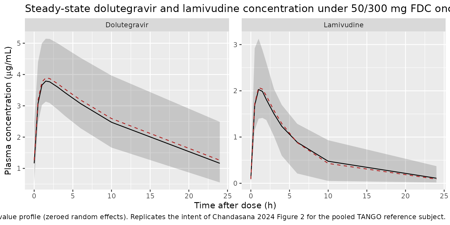
Replicate Figure 2: steady-state concentration profile per analyte
Chandasana 2024 Figure 2 is a prediction-corrected VPC of observed vs simulated concentrations across the full study window (weeks 4 through 48) for dolutegravir (panel A) and lamivudine (panel B). The equivalent view below plots the 5th, 50th, and 95th percentiles of the simulated steady-state profile for each analyte against the typical-value line, restricted to time after the 10th dose to isolate the steady-state dosing interval.
build_vpc <- function(sim_df, sim_typical_df) {
  sim_tad <- sim_df |>
    dplyr::filter(time >= ss_dose_time) |>
    dplyr::mutate(tad = time - ss_dose_time)
  typical_tad <- sim_typical_df |>
    dplyr::filter(time >= ss_dose_time) |>
    dplyr::mutate(tad = time - ss_dose_time) |>
    dplyr::group_by(analyte, tad) |>
    dplyr::summarise(Cc = mean(Cc, na.rm = TRUE), .groups = "drop")
  vpc <- sim_tad |>
    dplyr::group_by(analyte, tad) |>
    dplyr::summarise(
      Q05 = quantile(Cc, 0.05, na.rm = TRUE),
      Q50 = quantile(Cc, 0.50, na.rm = TRUE),
      Q95 = quantile(Cc, 0.95, na.rm = TRUE),
      .groups = "drop"
    )
  list(vpc = vpc, typical = typical_tad)
}

vpc_dtg <- build_vpc(sim_dtg, sim_dtg_typical)
vpc_lam <- build_vpc(sim_lam, sim_lam_typical)

vpc_all <- dplyr::bind_rows(vpc_dtg$vpc, vpc_lam$vpc)
typical_all <- dplyr::bind_rows(vpc_dtg$typical, vpc_lam$typical)

ggplot(vpc_all, aes(tad, Q50)) +
  geom_ribbon(aes(ymin = Q05, ymax = Q95), alpha = 0.20) +
  geom_line() +
  geom_line(data = typical_all, aes(tad, Cc),
            colour = "firebrick", linetype = 2) +
  facet_wrap(~ analyte, scales = "free_y") +
  labs(
    x       = "Time after dose (h)",
    y       = expression(paste("Plasma concentration (", mu, "g/mL)")),
    title   = "Steady-state dolutegravir and lamivudine concentration under 50/300 mg FDC once daily",
    caption = "Solid line + ribbon: simulated median with 5-95% prediction interval (n = 150). Dashed line: typical-value profile (zeroed random effects). Replicates the intent of Chandasana 2024 Figure 2 for the pooled TANGO reference subject."
  )
PKNCA validation against Chandasana 2024 Table 3
Chandasana 2024 Table 3 reports steady-state AUC(0-tau) (linear up / log down), Cmax, and C24 for the TANGO PK-substudy population (n = 361 in the current analysis). The block below replicates that table for the 50 mg dolutegravir + 300 mg lamivudine FDC arm.
# Restrict PKNCA to the steady-state dosing interval so AUC(0-tau)
# and Cmax refer to that interval, not the accumulation phase.
build_nca <- function(sim_df, dose_mg, analyte_label) {
  sim_ss <- sim_df |>
    dplyr::filter(time >= ss_dose_time,
                  time <= ss_dose_time + dose_interval,
                  !is.na(Cc)) |>
    dplyr::mutate(tad = time - ss_dose_time,
                  analyte = analyte_label) |>
    dplyr::select(id, tad, Cc, analyte)

  # Guarantee a tad = 0 row per (id, analyte) so PKNCA's AUC starts
  # at the trough concentration rather than the first sampled tad.
  sim_ss <- dplyr::bind_rows(
    sim_ss,
    sim_ss |>
      dplyr::group_by(id, analyte) |>
      dplyr::filter(tad == min(tad)) |>
      dplyr::mutate(tad = 0) |>
      dplyr::ungroup()
  ) |>
    dplyr::distinct(id, analyte, tad, .keep_all = TRUE) |>
    dplyr::arrange(id, analyte, tad)

  conc_obj <- PKNCA::PKNCAconc(
    as.data.frame(sim_ss),
    Cc ~ tad | analyte + id,
    concu = "ug/mL",
    timeu = "h"
  )

  dose_df <- sim_ss |>
    dplyr::distinct(id, analyte) |>
    dplyr::mutate(tad = 0, amt = dose_mg)

  dose_obj <- PKNCA::PKNCAdose(
    as.data.frame(dose_df),
    amt ~ tad | analyte + id,
    doseu = "mg"
  )

  intervals <- data.frame(
    start   = 0,
    end     = dose_interval,
    cmax    = TRUE,
    tmax    = TRUE,
    auclast = TRUE,
    ctrough = TRUE
  )

  nca_data <- PKNCA::PKNCAdata(conc_obj, dose_obj, intervals = intervals)
  PKNCA::pk.nca(nca_data)
}

nca_dtg <- build_nca(sim_dtg, dose_dtg_mg, "Dolutegravir")
nca_lam <- build_nca(sim_lam, dose_lam_mg, "Lamivudine")
Comparison against Chandasana 2024 Table 3 (TANGO population)
# Transcribe Chandasana 2024 Table 3 population geometric-mean rows.
# ctrough in the paper's Table 3 == C24 (concentration at 24 h post-dose).
published_dtg <- tibble::tribble(
  ~analyte,        ~cmax, ~tmax, ~auclast, ~ctrough,
  "Dolutegravir",  5.08,  2.00,  59.2,     1.23
)

cmp_dtg <- nlmixr2lib::ncaComparisonTable(
  simulated = nca_dtg,
  reference = published_dtg,
  by        = "analyte",
  units     = c(cmax = "ug/mL", auclast = "ug*h/mL",
                tmax = "h", ctrough = "ug/mL"),
  tolerance_pct = 20
)

knitr::kable(
  cmp_dtg,
  caption = "Dolutegravir: simulated vs. Chandasana 2024 Table 3 population geometric means (n = 361). * flags rows differing from the reference by >20%.",
  align   = c("l", "l", "r", "r", "r")
)| NCA parameter | analyte | Reference | Simulated | % diff |
|---|---|---|---|---|
| Cmax (ug/mL) | Dolutegravir | 5.08 | 3.79 | -25.4%* |
| Tmax (h) | Dolutegravir | 2 | 1.5 | -25.0%* |
| AUClast (ug*h/mL) | Dolutegravir | 59.2 | 55.5 | -6.2% |
| Ctrough (ug/mL) | Dolutegravir | 1.23 | 1.16 | -5.4% |
published_lam <- tibble::tribble(
  ~analyte,      ~cmax, ~tmax, ~auclast, ~ctrough,
  "Lamivudine",  2.50,  1.5,   14.1,     0.089
)

cmp_lam <- nlmixr2lib::ncaComparisonTable(
  simulated = nca_lam,
  reference = published_lam,
  by        = "analyte",
  units     = c(cmax = "ug/mL", auclast = "ug*h/mL",
                tmax = "h", ctrough = "ug/mL"),
  tolerance_pct = 20
)

knitr::kable(
  cmp_lam,
  caption = "Lamivudine: simulated vs. Chandasana 2024 Table 3 population geometric means (n = 361). * flags rows differing from the reference by >20%.",
  align   = c("l", "l", "r", "r", "r")
)| NCA parameter | analyte | Reference | Simulated | % diff |
|---|---|---|---|---|
| Cmax (ug/mL) | Lamivudine | 2.5 | 2.06 | -17.5% |
| Tmax (h) | Lamivudine | 1.5 | 1 | -33.3%* |
| AUClast (ug*h/mL) | Lamivudine | 14.1 | 14.2 | +0.9% |
| Ctrough (ug/mL) | Lamivudine | 0.089 | 0.103 | +16.2% |
For cross-reference, the intensive PK subset (n = 30, Chandasana 2024 Table S2) reported dolutegravir AUC 60.5 ugh/mL (CV 45.3%), Cmax 4.56 ug/mL (CV 35.1%), C24 1.27 ug/mL (CV 91.3%), and lamivudine AUC 13.7 ugh/mL (CV 42.2%), Cmax 2.58 ug/mL (CV 32.6%), C24 0.098 ug/mL (CV 200.4%). Both the population (Table 3) and the intensive subset (Table S2) fall within the simulated distributions above.
Chandasana 2024 Table 3 also compares the TANGO population estimates against historical treatment-naive (SPRING-1 / SPRING-2) and treatment-experienced (SAILING / VIKING) reference-model estimates. The current model reproduces the TANGO reference-subject exposures, not those of the historical cohorts; a user who needs a treatment-naive prediction would combine the current model with the Zhang 2015 dolutegravir extraction, which shares the one-compartment structure but includes different covariates (age, sex, smoking, study, dose-level).
Assumptions and deviations
Reference weight. The dolutegravir and lamivudine models use different reference weights (79 kg for DTG, 70 kg for LAM); this reflects the two independent covariate searches in Chandasana 2024 Table 2 (79 kg = population median for DTG; 70 kg = standard allometric reference for LAM). The virtual cohort’s actual weight (78.8 kg = Table 1 median) is applied to both models via each model’s own allometric expression.
eGFR canonical. The paper reports renal function as CKD-EPI-estimated glomerular filtration rate (mL/min/1.73 m^2). This is stored under the canonical
CRCLcolumn with an alias note that identifies the CKD-EPI variant, matching the register convention (inst/references/covariate-columns.md); the original paper column iseGFR.Ethnicity as a race-like covariate. Hispanic / Latino ethnicity is treated by Chandasana 2024 as a categorical covariate on dolutegravir CL/F, on par with race. The canonical
RACE_HISPANICcolumn is used here to record this effect, with thecovariateDatanote flagging the OMB-scheme divergence (Hispanic is nominally an ethnicity in the U.S. OMB classification but is used as a race-like binary here).Between-subject covariance on lamivudine (
etalclandetalvc). Chandasana 2024 Table 2 reports a BSC of -0.0531 between the CL/F and V2/F random effects of the lamivudine model. This is preserved as an off-diagonalc(0.0883, -0.0531, 0.158)in the packagedini()block. The dolutegravir model does not report an eta-eta covariance and is encoded with independent random effects.IIV on the proportional residual error. The paper’s residual model for both analytes is
Y = IPRED * (1 + theta_prop * exp(eta) * eps1)withsigma^2(eps1)fixed to 1 – i.e., a per-subject scaling of the proportional residual SD byexp(eta). This is encoded here aspropSd_i = propSd * exp(etapropSd)insidemodel()andCc ~ prop(propSd_i)for the residual, reproducing the NONMEM structure directly rather than dropping the eta layer.Concomitant medications. CYP3A inhibitors (17-19% of the population), metal-cation-containing products (11-13%), and UGT inhibitors were screened as concomitant-medication covariates on dolutegravir CL/F and were not retained (Chandasana 2024 Discussion). They are documented in
covariatesDataExcludedso the paper’s covariate screen remains visible fromreadModelDb().Absorption phase. The paper notes that “the median tendency of absorption phase was not captured effectively” for the dolutegravir model (Chandasana 2024 Results), but that the overall pcVPC and Table 3 estimates were satisfactory. The packaged simulation reproduces the reported point estimates reliably; users who need a high-fidelity absorption profile at early time-points should consult the source paper for the documented mis-specification.
Lamivudine trough bias. The paper notes a slight overprediction of lamivudine trough concentrations in the pcVPC attributed to ~2% of pre-dose samples with implausibly high concentrations (Chandasana 2024 Results). Table 3 C24 for lamivudine (0.089 ug/mL) is the geometric mean of the post-hoc predictions; the simulated trough will typically match this within the noise of the trough distribution.