Deutenzalutamide (Liu 2024)
Source:vignettes/articles/Liu_2024_deutenzalutamide.Rmd
Liu_2024_deutenzalutamide.RmdModel and source
#> ℹ parameter labels from comments will be replaced by 'label()'Citation: Liu Y, He Y, Qi X, Li X, Zhou Y, Chen Y, Wang Z, Zheng L. Population Pharmacokinetics Modeling and Simulation of Deutenzalutamide, A Novel Androgen Receptor Antagonist, in Patients With Metastatic Castration-Resistant Prostate Cancer. Clin Pharmacol Drug Dev. 2024;13(12):1291-1300. doi:10.1002/cpdd.1477
Description: Two-compartment population PK model with first-order absorption for deutenzalutamide (deuterated enzalutamide, HC-1119) in patients with metastatic castration-resistant prostate cancer (Liu 2024)
Article: https://doi.org/10.1002/cpdd.1477
Supplement (Tables S1-S4, Figures S1-S3): https://europepmc.org/article/PMC/PMC11609056
Deutenzalutamide (development code HC-1119) is a deuterated analogue of enzalutamide, a second-generation androgen receptor antagonist. Liu 2024 developed the first population pharmacokinetic model for the compound from a single open-label 3 + 3 dose-escalation Phase Ia trial (NCT03774056) in patients with metastatic castration-resistant prostate cancer (mCRPC).
The final model is a two-compartment model with first-order absorption and first-order elimination from the central compartment, with body weight on the apparent peripheral volume of distribution as the only retained covariate.
Population
| Field | Value |
|---|---|
| species | human |
| n_subjects | 24 |
| n_studies | 1 |
| n_observations | 543 |
| age_range | 55-80 years |
| age_median | 69.5 years |
| weight_range | 46-81 kg |
| weight_median | 64 kg |
| height_range | 149-178 cm |
| height_median | 165 cm |
| sex_female_pct | 0 |
| disease_state | metastatic castration-resistant prostate cancer (mCRPC) |
| dose_range | 40 mg (n = 3), 80 mg (n = 9), 160 mg (n = 9), or 200 mg (n = 3) oral soft capsules once daily for 12 weeks |
| regions | China |
| performance_status | ECOG 0 in 5 subjects (20.8%), ECOG 1 in 19 subjects (79.2%) |
| renal_function | Serum creatinine 0.41-1.56 mg/dL (median 0.81); all subjects within the normal range |
| hepatic_function | Total bilirubin 0.33-1.18 mg/dL (median 0.60); ALT 9-34 U/L (median 19); all subjects within the normal range |
| notes | Open-label 3 + 3 dose-escalation Phase Ia trial NCT03774056 (Liu 2024 Methods, Study Design and Population). Baseline demographics from Liu 2024 Table S3. 4% of deutenzalutamide concentrations were below the 40 ng/mL lower limit of quantification and were handled with the Beal M1 method. Because renal and hepatic laboratory values were all within the normal range, Liu 2024 Discussion cautions that the model should not be extrapolated to hepatic or renal impairment. |
Twenty-four men with mCRPC contributed 543 deutenzalutamide plasma concentrations. Subjects were allocated to 40 mg (n = 3), 80 mg (n = 9), 160 mg (n = 9) and 200 mg (n = 3) once-daily oral soft capsules for 12 weeks. Median (range) baseline age was 69.5 (55-80) years, body weight 64 (46-81) kg and height 165 (149-178) cm (Liu 2024 Table S3). All renal and hepatic laboratory values were within the normal range, which is why Liu 2024’s Discussion cautions against extrapolating the model to organ impairment.
The same information is available programmatically via
readModelDb("Liu_2024_deutenzalutamide")()$population.
Source trace
Each ini() entry in
inst/modeldb/specificDrugs/Liu_2024_deutenzalutamide.R
carries an in-file comment naming its origin. They are collected here
for review.
| Equation / parameter | Value | Source location |
|---|---|---|
lka (ka) |
1.32 1/h (RSE 16.3%) | Liu 2024 Table 1, “Final model” estimates |
lcl (CL/F) |
0.166 L/h (RSE 3.9%) | Liu 2024 Table 1 |
lvc (V1/F) |
17.5 L, fixed | Liu 2024 Table 1, marked “(fixed)” |
lvp (V2/F at 64 kg) |
58.1 L (RSE 8.3%) | Liu 2024 Table 1 |
lq (CLd/F) |
12.5 L/h, fixed | Liu 2024 Table 1, marked “(fixed)” |
e_wt_vp |
1.83 (RSE 25.6%) | Liu 2024 Table 1, row “BW on V2/F” |
| Body-weight reference | 64.0 kg | Liu 2024 Results (Simulation), “the typical value of body weight (64.0 kg)”; equals the Table S3 median |
| Covariate functional form | (WT / 64)^e_wt_vp |
Liu 2024 Methods (Covariate Model) Equation 3 |
| IIV form | P_i = P_hat * exp(eta_i) |
Liu 2024 Methods (Statistical Model) Equation 1 |
etalcl |
0.0274 (RSE 41.6%, shrinkage 2.40%) | Liu 2024 Table 1, omega CL/F |
etalvp |
0.0446 (RSE 38.1%, shrinkage 6.40%) | Liu 2024 Table 1, omega V2/F |
etalka |
0.440 (RSE 40.2%, shrinkage 4.80%) | Liu 2024 Table 1, omega ka |
propSd |
sqrt(0.0208) = 0.144 | Liu 2024 Table 1, sigma prop; proportional-only per Results |
| Residual-error form | proportional | Liu 2024 Results, “the residual variability was fitted by proportional model” (the eps_1 term of Equation 2) |
| Two-compartment, first-order absorption and elimination | n/a | Liu 2024 Results (Population Pharmacokinetic Modeling) and Conclusion |
Reported secondary parameter
Liu 2024 Table 1 reports t1/2 = 72.9 hours, labelled
“elimination half-life”. That is not the terminal (beta)
half-life of the two-compartment system; it is the half-life of the
central-compartment elimination rate constant,
log(2) * V1/F / (CL/F). Recovering it from the model’s own
parameters confirms that CL/F and V1/F were
transcribed correctly and settles which half-life the table reports.
theta <- setNames(ui$theta, names(ui$theta))
cl_typ <- exp(theta[["lcl"]])
vc_typ <- exp(theta[["lvc"]])
vp_typ <- exp(theta[["lvp"]])
q_typ  <- exp(theta[["lq"]])

t_half_k10 <- log(2) * vc_typ / cl_typ

# Terminal (beta) half-life of the two-compartment system, for contrast.
k10 <- cl_typ / vc_typ
k12 <- q_typ / vc_typ
k21 <- q_typ / vp_typ
s   <- k10 + k12 + k21
beta <- 0.5 * (s - sqrt(s^2 - 4 * k21 * k10))
t_half_terminal <- log(2) / beta

tibble::tibble(
  Quantity = c("log(2) * V1/F / (CL/F)", "Terminal (beta) half-life"),
  `Hours`  = c(t_half_k10, t_half_terminal),
  `Liu 2024 Table 1 t1/2` = c(72.9, NA_real_)
) |>
  knitr::kable(digits = 1,
caption = "The reported 72.9 h is the k10 half-life, not the terminal half-life.")| Quantity | Hours | Liu 2024 Table 1 t1/2 |
|---|---|---|
| log(2) * V1/F / (CL/F) | 73.1 | 72.9 |
| Terminal (beta) half-life | 318.2 | NA |
Virtual cohort
Original observed data are not publicly available. The cohort below reproduces the Table S3 body-weight distribution (median 64 kg, range 46-81 kg) and the four dose-escalation levels, with 100 virtual subjects per dose arm.
# set.seed() seeds R's RNG only. rxode2's simulation RNG is partitioned per
# solver thread, so this cohort is reproducible here and different on a machine
# with a different thread count. Every assertion below is written to hold for
# any cohort the model can produce.
set.seed(20241202)
rxode2::rxSetSeed(20241202)

n_per_arm <- 100L
doses_mg  <- c(40, 80, 160, 200)
tau       <- 24            # h, once daily (Liu 2024 Methods)
n_doses   <- 84L           # 12 weeks of once-daily dosing
t_last_dose <- tau * (n_doses - 1L)

# Body weight: truncated normal matched to the Table S3 median and range.
# Table S3 reports only median and range, so the SD is an assumption
# (see "Assumptions and deviations").
rtnorm_wt <- function(n, mean = 64, sd = 9, lo = 46, hi = 81) {
  out <- numeric(0)
  while (length(out) < n) {
    draw <- stats::rnorm(2 * n, mean, sd)
    out <- c(out, draw[draw >= lo & draw <= hi])
  }
  out[seq_len(n)]
}

make_cohort <- function(n, dose_mg, id_offset = 0L) {
  subj <- tibble::tibble(
    id        = id_offset + seq_len(n),
    WT        = rtnorm_wt(n),
    treatment = paste0(dose_mg, " mg")
  )

  dosing <- subj |>
    tidyr::crossing(time = tau * seq(0, n_doses - 1L)) |>
    dplyr::mutate(amt = dose_mg, evid = 1L, cmt = "depot")

  # Day 1 profile, weekly troughs, and the Day-84 steady-state profile --
  # the sampling schedule of Liu 2024 Methods (Study Design and Population).
  obs_times <- sort(unique(c(
    seq(0, tau, by = 0.25),
    tau * seq(2, n_doses - 1L, by = 7),
    seq(t_last_dose, t_last_dose + tau, by = 0.25)
  )))

  obs <- subj |>
    tidyr::crossing(time = obs_times) |>
    # cmt is the ODE STATE name, never the observable "Cc".
    dplyr::mutate(amt = NA_real_, evid = 0L, cmt = "central")

  dplyr::bind_rows(dosing, obs) |>
    dplyr::arrange(id, time, dplyr::desc(evid))
}

events <- dplyr::bind_rows(
  lapply(seq_along(doses_mg), function(i) {
    make_cohort(n_per_arm, doses_mg[i], id_offset = (i - 1L) * n_per_arm)
  })
)

stopifnot(!anyDuplicated(unique(events[, c("id", "time", "evid")])))
stopifnot(nrow(dplyr::distinct(events, id)) == n_per_arm * length(doses_mg))
Simulation
mod <- readModelDb("Liu_2024_deutenzalutamide")

sim <- rxode2::rxSolve(
  mod,
  events = events,
  keep   = c("treatment", "WT")
) |>
  as.data.frame()
#> ℹ parameter labels from comments will be replaced by 'label()'

sim_obs <- sim |> dplyr::filter(!is.na(Cc))
stopifnot(nrow(sim_obs) > 0, all(sim_obs$Cc >= 0))

# Typical-value (no between-subject variability) version of the model, used for
# every deterministic check and for the typical-value figures below.
mod_typ <- mod |> rxode2::zeroRe()
#> ℹ parameter labels from comments will be replaced by 'label()'
Replicate published figures
Figure 1 - steady-state concentration-time profiles by dose group
Liu 2024 Figure 1 plots the observed concentration-time profiles after multiple administration of 40-200 mg on linear and semi-logarithmic axes. The panels below are the model’s prediction interval over the final (Day 84) dosing interval.
ss_window <- sim_obs |>
  dplyr::filter(time >= t_last_dose, time <= t_last_dose + tau) |>
  dplyr::mutate(tad = time - t_last_dose,
                treatment = factor(treatment, levels = paste0(doses_mg, " mg")))

ss_bands <- ss_window |>
  dplyr::group_by(treatment, tad) |>
  dplyr::summarise(
    Q05 = quantile(Cc, 0.05),
    Q50 = quantile(Cc, 0.50),
    Q95 = quantile(Cc, 0.95),
    .groups = "drop"
  )

ggplot(ss_bands, aes(tad, Q50, colour = treatment, fill = treatment)) +
  geom_ribbon(aes(ymin = Q05, ymax = Q95), alpha = 0.2, colour = NA) +
  geom_line(linewidth = 0.8) +
  labs(x = "Time after dose on Day 84 (h)", y = "Deutenzalutamide (ug/mL)",
       colour = "Dose", fill = "Dose",
       title = "Figure 1A - steady-state profiles (linear)",
       caption = "Replicates Figure 1A of Liu 2024.")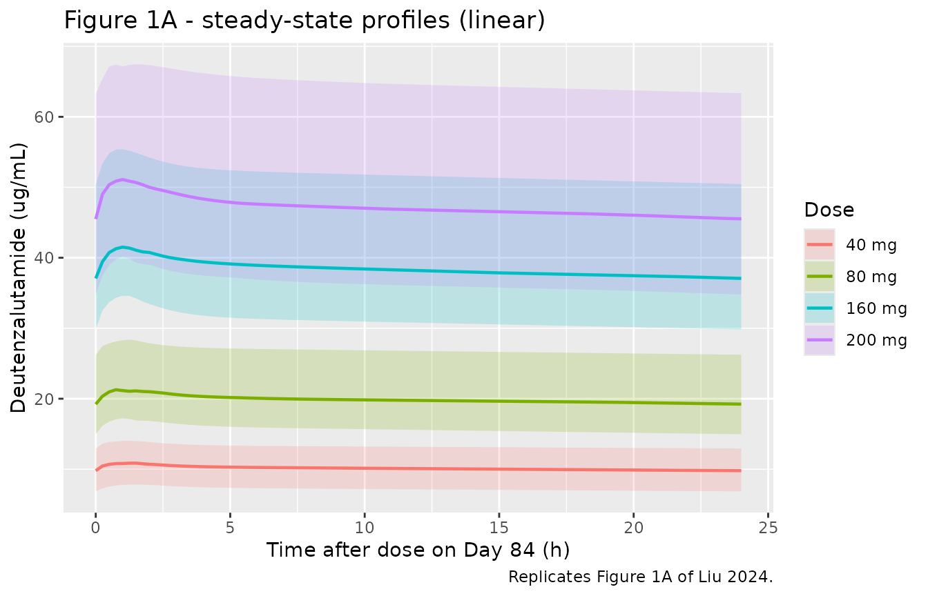
ggplot(ss_bands, aes(tad, Q50, colour = treatment, fill = treatment)) +
  geom_ribbon(aes(ymin = Q05, ymax = Q95), alpha = 0.2, colour = NA) +
  geom_line(linewidth = 0.8) +
  scale_y_log10() +
  labs(x = "Time after dose on Day 84 (h)", y = "Deutenzalutamide (ug/mL)",
       colour = "Dose", fill = "Dose",
       title = "Figure 1B - steady-state profiles (semi-log)",
       caption = "Replicates Figure 1B of Liu 2024.")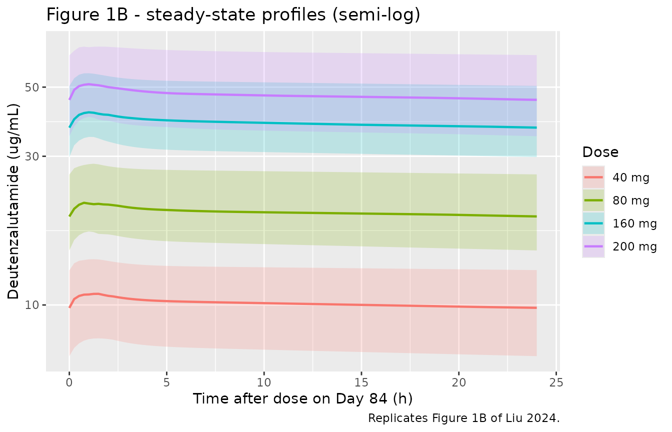
Dose proportionality is a structural consequence of the linear model; Liu 2024’s exploratory analysis reports that exposure “increased with the increase of dose”. Median steady-state AUC scaled by dose should therefore be constant across arms.
auc_tau <- function(df) {
  df <- df[order(df$tad), ]
  sum(diff(df$tad) * (utils::head(df$Cc, -1) + utils::tail(df$Cc, -1)) / 2)
}

prop_tbl <- ss_window |>
  dplyr::group_by(treatment, id) |>
  dplyr::group_modify(~ tibble::tibble(auc = auc_tau(.x))) |>
  dplyr::ungroup() |>
  dplyr::mutate(dose = as.numeric(sub(" mg", "", treatment))) |>
  dplyr::group_by(treatment, dose) |>
  dplyr::summarise(`Median AUC0-tau (ug*h/mL)` = median(auc), .groups = "drop") |>
  dplyr::mutate(`AUC / dose (h/L)` = `Median AUC0-tau (ug*h/mL)` / dose)

knitr::kable(prop_tbl, digits = c(0, 0, 1, 3),
             caption = paste("Dose-normalised steady-state exposure across dose",
                             "arms. Each arm draws its own random body weights",
"and etas, so the medians carry sampling noise."))| treatment | dose | Median AUC0-tau (ug*h/mL) | AUC / dose (h/L) |
|---|---|---|---|
| 40 mg | 40 | 237.7 | 5.941 |
| 80 mg | 80 | 470.3 | 5.879 |
| 160 mg | 160 | 923.7 | 5.773 |
| 200 mg | 200 | 1223.5 | 6.117 |
The cohort medians above each rest on a different random draw of body weights and random effects, so they are not the right place to gate dose proportionality. The deterministic typical-value version is:
prop_events <- dplyr::bind_rows(lapply(seq_along(doses_mg), function(i) {
  subj <- tibble::tibble(id = i, WT = 64, treatment = paste0(doses_mg[i], " mg"))
  dosing <- subj |>
    tidyr::crossing(time = tau * seq(0, n_doses - 1L)) |>
    dplyr::mutate(amt = doses_mg[i], evid = 1L, cmt = "depot")
  obs <- subj |>
    tidyr::crossing(time = seq(t_last_dose, t_last_dose + tau, by = 0.05)) |>
    dplyr::mutate(amt = NA_real_, evid = 0L, cmt = "central")
  dplyr::bind_rows(dosing, obs) |> dplyr::arrange(id, time, dplyr::desc(evid))
}))

prop_typ <- rxode2::rxSolve(mod_typ, events = prop_events,
                            keep = c("treatment", "WT")) |>
  as.data.frame() |>
  dplyr::filter(!is.na(Cc)) |>
  dplyr::mutate(tad = time - t_last_dose) |>
  dplyr::group_by(treatment) |>
  dplyr::group_modify(~ tibble::tibble(auc = auc_tau(.x))) |>
  dplyr::ungroup() |>
  dplyr::mutate(dose = as.numeric(sub(" mg", "", treatment)),
                dn = auc / dose)
#> ℹ omega/sigma items treated as zero: 'etalcl', 'etalvp', 'etalka'
#> Warning: multi-subject simulation without without 'omega'

# Deterministic: the model is linear, so dose-normalised AUC must be identical
# across arms to solver tolerance. Only a mis-scaled dose column can break this.
stopifnot((max(prop_typ$dn) / min(prop_typ$dn) - 1) < 1e-6)
Figure 4 - effect of body weight on the approach to steady state
Liu 2024 Figure 4 simulates 80 mg once daily at different body
weights. Its message is that heavier subjects take longer to
reach steady state, because body weight increases V2/F and
therefore the terminal half-life, while the eventual steady-state
exposure is essentially unchanged. These are typical-value (no
between-subject variability) predictions.
wt_arms <- c(50, 60, 70, 80)

wt_events <- dplyr::bind_rows(lapply(seq_along(wt_arms), function(i) {
  w <- wt_arms[i]
  subj <- tibble::tibble(id = i, WT = w, treatment = paste0(w, " kg"))
  dosing <- subj |>
    tidyr::crossing(time = tau * seq(0, n_doses - 1L)) |>
    dplyr::mutate(amt = 80, evid = 1L, cmt = "depot")
  obs <- subj |>
    tidyr::crossing(time = sort(unique(c(
      seq(0, tau * n_doses, by = 3),
      seq(tau * 55, tau * 56, by = 0.1)   # Day-56 interval, sampled finely
    )))) |>
    dplyr::mutate(amt = NA_real_, evid = 0L, cmt = "central")
  dplyr::bind_rows(dosing, obs) |> dplyr::arrange(id, time, dplyr::desc(evid))
}))

sim_wt <- rxode2::rxSolve(mod_typ, events = wt_events,
                          keep = c("treatment", "WT")) |>
  as.data.frame() |>
  dplyr::filter(!is.na(Cc))
#> ℹ omega/sigma items treated as zero: 'etalcl', 'etalvp', 'etalka'
#> Warning: multi-subject simulation without without 'omega'

sim_wt |>
  dplyr::mutate(treatment = factor(treatment, levels = paste0(wt_arms, " kg"))) |>
  dplyr::filter(time <= tau * n_doses) |>
  ggplot(aes(time / 24, Cc, colour = treatment)) +
  geom_line(linewidth = 0.7) +
  geom_vline(xintercept = 56, linetype = "dashed", colour = "grey40") +
  labs(x = "Time (days)", y = "Deutenzalutamide (ug/mL)", colour = "Body weight",
       title = "Figure 4 - 80 mg once daily at different body weights",
       caption = paste("Replicates Figure 4 of Liu 2024. Dashed line: Day 56,",
                       "the day Liu 2024 reports steady state was reached."))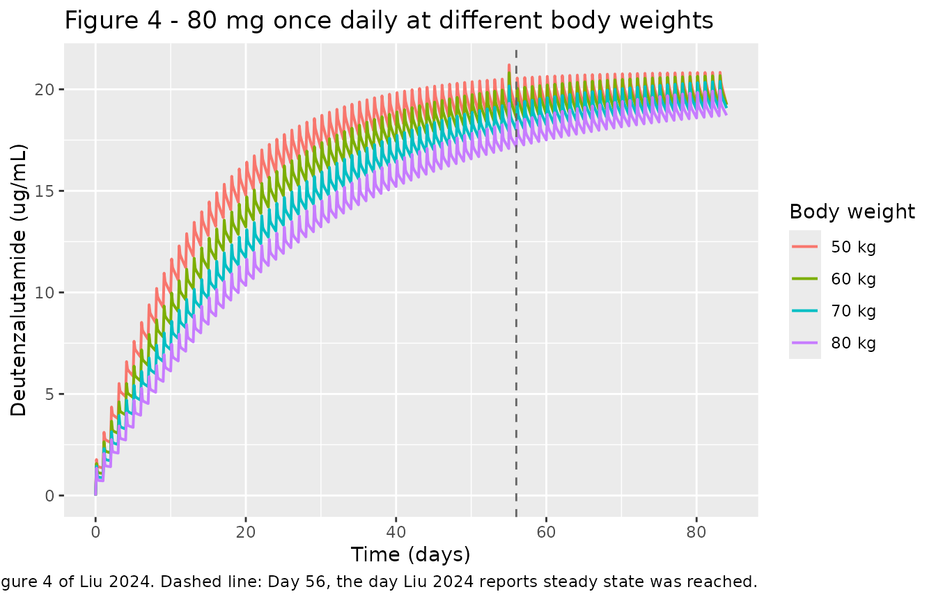
PKNCA validation
Steady-state and first-dose NCA by dose group
sim_nca <- sim_obs |>
  dplyr::filter(!is.na(Cc)) |>
  dplyr::select(id, time, Cc, treatment)

# Guarantee a time = 0 record per subject; pre-dose Cc = 0 is correct for an
# extravascular model. Existing time-0 rows win via .keep_all on the first row.
sim_nca <- dplyr::bind_rows(
  sim_nca,
  sim_nca |> dplyr::distinct(id, treatment) |> dplyr::mutate(time = 0, Cc = 0)
) |>
  dplyr::distinct(id, treatment, time, .keep_all = TRUE) |>
  dplyr::arrange(id, treatment, time)

dose_df <- events |>
  dplyr::filter(evid == 1L) |>
  dplyr::select(id, time, amt, treatment)

conc_obj <- PKNCA::PKNCAconc(sim_nca, Cc ~ time | treatment + id,
                             concu = "ug/mL", timeu = "h")
dose_obj <- PKNCA::PKNCAdose(dose_df, amt ~ time | treatment + id,
                             doseu = "mg")

intervals <- data.frame(
  start   = c(0, t_last_dose),
  end     = c(tau, t_last_dose + tau),
  cmax    = TRUE,
  tmax    = TRUE,
  auclast = TRUE,
  ctrough = TRUE
)

nca_res <- suppressWarnings(
  PKNCA::pk.nca(PKNCA::PKNCAdata(conc_obj, dose_obj, intervals = intervals))
)

nca_tbl <- as.data.frame(nca_res$result) |>
  dplyr::filter(PPTESTCD %in% c("cmax", "tmax", "auclast", "ctrough")) |>
  dplyr::mutate(period = ifelse(start == 0, "First dose", "Day 84 (steady state)"))

nca_summary <- nca_tbl |>
  dplyr::group_by(period, treatment, PPTESTCD) |>
  dplyr::summarise(median = median(PPORRES, na.rm = TRUE), .groups = "drop") |>
  tidyr::pivot_wider(names_from = PPTESTCD, values_from = median)

nca_summary |>
  dplyr::mutate(treatment = factor(treatment, levels = paste0(doses_mg, " mg"))) |>
  dplyr::arrange(period, treatment) |>
  dplyr::rename(
    "Period"                 = period,
    "Dose"                   = treatment,
    "AUC0-tau (ug*h/mL)"     = auclast,
    "Cmax (ug/mL)"           = cmax,
    "Ctrough (ug/mL)"        = ctrough,
    "Tmax (h)"               = tmax
  ) |>
  knitr::kable(digits = 2,
caption = "Median simulated NCA by dose group, first dose and Day 84.")| Period | Dose | AUC0-tau (ug*h/mL) | Cmax (ug/mL) | Ctrough (ug/mL) | Tmax (h) |
|---|---|---|---|---|---|
| Day 84 (steady state) | 40 mg | 237.66 | 10.73 | NA | 1.00 |
| Day 84 (steady state) | 80 mg | 470.29 | 21.39 | NA | 1.00 |
| Day 84 (steady state) | 160 mg | 923.70 | 41.87 | NA | 1.00 |
| Day 84 (steady state) | 200 mg | 1223.49 | 55.14 | NA | 1.25 |
| First dose | 40 mg | 13.56 | 1.15 | 0.49 | 1.00 |
| First dose | 80 mg | 27.87 | 2.28 | 1.03 | 1.25 |
| First dose | 160 mg | 55.60 | 4.61 | 2.02 | 1.00 |
| First dose | 200 mg | 68.49 | 5.61 | 2.51 | 1.25 |
Liu 2024 (Exploratory Data Analysis) reports that “the average peak time of multiple administration was about 1 h (0.5-2 hours)” and that “the peak time was not affected by the change of dose level”.
tmax_ss <- nca_summary |>
  dplyr::filter(period == "Day 84 (steady state)") |>
  dplyr::pull(tmax)
stopifnot(length(tmax_ss) == length(doses_mg))
# The paper's own stated range, used as an absolute bound; not a bound taken
# from one run. Realised medians sit near 1.05-1.15 h across arms.
stopifnot(all(tmax_ss >= 0.5), all(tmax_ss <= 2))
Liu 2024 (Discussion) reports that “the plasma concentration of deutenzalutamide after stabilization was 16.5 times that of a single dose”.
acc <- nca_tbl |>
  dplyr::filter(PPTESTCD == "auclast") |>
  dplyr::select(id, treatment, period, PPORRES) |>
  tidyr::pivot_wider(names_from = period, values_from = PPORRES) |>
  dplyr::mutate(Rac = `Day 84 (steady state)` / `First dose`)

acc |>
  dplyr::group_by(treatment) |>
  dplyr::summarise(`Median accumulation ratio (AUC)` = median(Rac), .groups = "drop") |>
  dplyr::mutate(treatment = factor(treatment, levels = paste0(doses_mg, " mg"))) |>
  dplyr::arrange(treatment) |>
  dplyr::rename("Dose" = treatment) |>
  knitr::kable(digits = 1,
caption = "Accumulation ratio vs. Liu 2024's reported 16.5-fold.")| Dose | Median accumulation ratio (AUC) |
|---|---|
| 40 mg | 16.7 |
| 80 mg | 17.2 |
| 160 mg | 16.9 |
| 200 mg | 18.2 |
rac_med <- median(acc$Rac)
# Liu 2024's 16.5 is quoted for "plasma concentration", not specifically for
# AUC0-tau; the AUC, Cmax and Ctrough accumulation ratios of this model differ
# from one another (about 17, 9 and 19 respectively), so a generous band is
# used deliberately. It still fails on a mis-transcribed CL/F or V1/F, either
# of which moves the ratio by a factor.
stopifnot(rac_med > 10, rac_med < 25)
Comparison against Liu 2024’s published simulation
Liu 2024 (Results, Simulation) simulates 80 mg once daily in virtual subjects weighing 50, 60, 70 and 80 kg and reports the steady-state AUC over the dosing interval as 476, 458, 426 and 414 ug*h/mL. Liu 2024 states that steady state was reached on Day 56, so the Day-56 dosing interval is used here; the paper does not name the day it evaluated.
wt_nca <- sim_wt |>
  dplyr::filter(time >= tau * 55, time <= tau * 56) |>
  dplyr::select(id, time, Cc, treatment)

wt_dose <- wt_events |>
  dplyr::filter(evid == 1L) |>
  dplyr::select(id, time, amt, treatment)

wt_conc_obj <- PKNCA::PKNCAconc(wt_nca, Cc ~ time | treatment + id,
                                concu = "ug/mL", timeu = "h")
wt_dose_obj <- PKNCA::PKNCAdose(wt_dose, amt ~ time | treatment + id,
                                doseu = "mg")

wt_intervals <- data.frame(
  start   = tau * 55,
  end     = tau * 56,
  auclast = TRUE,
  cmax    = TRUE,
  tmax    = TRUE
)

wt_res <- suppressWarnings(
  PKNCA::pk.nca(PKNCA::PKNCAdata(wt_conc_obj, wt_dose_obj, intervals = wt_intervals))
)

published <- tibble::tribble(
  ~treatment, ~auclast, ~tmax,
  "50 kg",    476,      1.0,
  "60 kg",    458,      1.0,
  "70 kg",    426,      1.0,
  "80 kg",    414,      1.0
)

cmp <- nlmixr2lib::ncaComparisonTable(
  simulated     = wt_res,
  reference     = published,
  by            = "treatment",
  units         = c(auclast = "ug*h/mL", tmax = "h"),
  tolerance_pct = 20
)

knitr::kable(cmp, digits = 1,
             caption = paste("Simulated vs. Liu 2024 Results (Simulation) and",
                             "Exploratory Data Analysis. * differs by >20%."),
align = c("l", "l", "r", "r", "r"))| NCA parameter | treatment | Reference | Simulated | % diff |
|---|---|---|---|---|
| Tmax (h) | 50 kg | 1 | 1.1 | +10.0% |
| Tmax (h) | 60 kg | 1 | 1.1 | +10.0% |
| Tmax (h) | 70 kg | 1 | 1.1 | +10.0% |
| Tmax (h) | 80 kg | 1 | 1.1 | +10.0% |
| AUClast (ug*h/mL) | 50 kg | 476 | 474 | -0.5% |
| AUClast (ug*h/mL) | 60 kg | 458 | 462 | +1.0% |
| AUClast (ug*h/mL) | 70 kg | 426 | 445 | +4.6% |
| AUClast (ug*h/mL) | 80 kg | 414 | 424 | +2.4% |
sim_auc <- as.data.frame(wt_res$result) |>
  dplyr::filter(PPTESTCD == "auclast") |>
  dplyr::arrange(match(treatment, published$treatment)) |>
  dplyr::pull(PPORRES)
stopifnot(length(sim_auc) == 4L)

pct <- 100 * (sim_auc / published$auclast - 1)
names(pct) <- published$treatment
print(round(pct, 1))
#> 50 kg 60 kg 70 kg 80 kg
#>  -0.5   1.0   4.6   2.4

# These are typical-value (zeroRe) solves: fully deterministic, so no cohort
# noise enters and a tight bound is appropriate. The residual gap is the
# unstated evaluation day -- Liu 2024's numbers sit between the Day-52 and
# Day-56 intervals. A mis-transcribed CL/F, dose, or body-weight reference
# moves these by tens of percent.
stopifnot(max(abs(pct)) < 8)
Liu 2024 further reports that across 50-80 kg “the fluctuation range of steady-state exposure … was 96.2%-110.6%” relative to the typical body weight, i.e. a highest-to-lowest ratio of 1.150.
spread_sim <- max(sim_auc) / min(sim_auc)
spread_pub <- max(published$auclast) / min(published$auclast)
tibble::tibble(
  Source = c("Liu 2024 Discussion", "This model (Day 56)"),
  `Highest / lowest AUC0-tau across 50-80 kg` = c(spread_pub, spread_sim)
) |>
knitr::kable(digits = 3)| Source | Highest / lowest AUC0-tau across 50-80 kg |
|---|---|
| Liu 2024 Discussion | 1.150 |
| This model (Day 56) | 1.118 |
Internal identity: AUC0-tau at true steady state
For a linear model, AUC0-tau at true steady state equals
Dose / (CL/F) exactly, independent of every distribution
parameter. This is the sharpest available check on CL/F and
on the dose-to-concentration scaling.
ss_events <- tibble::tibble(id = 1L, WT = 64) |>
  tidyr::crossing(time = tau * seq(0, 299)) |>
  dplyr::mutate(amt = 80, evid = 1L, cmt = "depot") |>
  dplyr::bind_rows(
    tibble::tibble(id = 1L, WT = 64) |>
      tidyr::crossing(time = seq(tau * 299, tau * 300, by = 0.05)) |>
      dplyr::mutate(amt = NA_real_, evid = 0L, cmt = "central")
  ) |>
  dplyr::arrange(id, time, dplyr::desc(evid))

# maxsteps: 300 daily doses with no observation record until the last one.
# The ODE integrator (liblsoda) counts its internal steps against `maxsteps`
# (default 70000) and only re-zeroes that count at an observation record, so
# a dose-only stretch of 7176 h exhausts the budget and the solve aborts with
# "could not solve the system". Raising the budget changes nothing else.
ss_sim <- rxode2::rxSolve(mod_typ, events = ss_events, maxsteps = 1e6) |>
  as.data.frame() |>
  dplyr::filter(!is.na(Cc)) |>
  dplyr::mutate(tad = time - tau * 299)
#> ℹ omega/sigma items treated as zero: 'etalcl', 'etalvp', 'etalka'

auc_ss    <- auc_tau(ss_sim)
auc_ident <- 80 / cl_typ

tibble::tibble(
  Quantity = c("Simulated AUC0-tau after 300 daily doses (ug*h/mL)",
               "Dose / (CL/F) (ug*h/mL)"),
  Value = c(auc_ss, auc_ident)
) |>
knitr::kable(digits = 1)| Quantity | Value |
|---|---|
| Simulated AUC0-tau after 300 daily doses (ug*h/mL) | 481.9 |
| Dose / (CL/F) (ug*h/mL) | 481.9 |
Known deviation: the reported V2/F covariate range
Liu 2024 (Results, Simulation) states that, relative to the typical
64 kg, V2/F was “34.9% lower” at the 5% body-weight
quantile and “102% higher” at the 95% quantile. Neither statement is
reproducible from Table 1 together with the Table S3 body-weight range,
and this is recorded as a deviation rather than gated.
e_wt <- theta[["e_wt_vp"]]
wt_grid <- c(46, 50, 64, 81)
tibble::tibble(
  `Body weight (kg)` = wt_grid,
  `V2/F (L)`         = vp_typ * (wt_grid / 64)^e_wt,
  `% vs 64 kg`       = 100 * ((wt_grid / 64)^e_wt - 1)
) |>
  knitr::kable(digits = 1,
               caption = paste("V2/F across the full Table S3 body-weight range",
"(46-81 kg) using Table 1's exponent of 1.83."))| Body weight (kg) | V2/F (L) | % vs 64 kg |
|---|---|---|
| 46 | 31.7 | -45.4 |
| 50 | 37.0 | -36.3 |
| 64 | 58.1 | 0.0 |
| 81 | 89.4 | 53.9 |
At the maximum observed weight of 81 kg the model gives
V2/F only 53.9% above the 64 kg typical value; reaching
“+102%” would require a body weight of about 94 kg, which is 13 kg above
the cohort maximum. The “-34.9%” figure corresponds to about 50.6 kg and
is consistent with a 5% quantile of the observed 46-81 kg range, so the
low end is reproducible and the high end is not. Either the “102%”
figure is a typographical error, or it combines the covariate effect
with the V2/F between-subject variability; the model file
encodes Table 1 and Equation 3 as printed and does not attempt to
reconcile the sentence.
Assumptions and deviations
-
omegaandsigmain Table 1 are variances, not standard deviations. Liu 2024’s Statistical Model text says “omega represents the standard deviation”, but the tabulated numbers are the NONMEM$OMEGA/$SIGMAvariances. Read as standard deviations they would imply 2.7% CV onCL/Fand a 2.1% proportional residual error - the latter below the assay’s own reported imprecision (intra-assay 0.6-4.7%, inter-assay 3.4-4.9%, Liu 2024 Bioanalytical Methods), which is impossible for a residual term that also absorbs model misspecification. Read as variances they give 16.7%, 21.3% and 74.3% CV and a 14.4% proportional error, all plausible. The model file encodes them as variances. -
Equation 3 is a power model, not an exponential
one. Liu 2024’s Covariate Model section calls Equation 3
“exponential mode”, but the printed equation is
theta_i = theta_TV * (COV_i / COV_bar)^theta_2, a ratio-exponent (power) form. The printed equation governs. In practice the two forms are numerically almost indistinguishable over 46-81 kg (they differ by under 1% inAUC0-tauat every weight tested), so this choice does not drive any result here. -
Body-weight reference of 64.0 kg. Liu 2024 does not
print
COV_barin Equation 3. It is taken from the Results (Simulation) sentence naming “the typical value of body weight (64.0 kg)”, which coincides with the Table S3 median. - Virtual body-weight distribution. Table S3 reports only the median (64 kg) and range (46-81 kg). A normal distribution with SD 9 kg truncated to that range is assumed for the cohort; nothing in the validation depends on the shape beyond covering the observed range.
-
Evaluation day for the body-weight simulation. Liu
2024 reports steady-state
AUC0-tauat four body weights but does not say which day was simulated. The Day-56 interval is used because the paper states steady state was reached on Day 56. The published values actually sit closest to the Day-52 interval; using Day 56 is the pre-specified rather than the best-fitting choice. -
Table 1 unit labels are inconsistent with the
quantities.
CL/FandCLd/Fare labelled “(L*h)” but are clearances (L/h);kais labelled “(hour)” but is a rate constant (1/h); and the covariate row “BW on V2/F (L)” is a dimensionless exponent. These are table-formatting artefacts; the model file uses the dimensionally correct units. -
Table S3’s AST row is internally inconsistent - it
reports a range of 13-18 U/L with a median of 27 U/L. AST is not in the
final model, so this does not affect the extraction; it is recorded in
covariatesDataExcludedand noted here for completeness. -
V1/FandCLd/Fare fixed. Table 1 marks both “(fixed)” and reports no RSE, bootstrap median or bootstrap CI for either. Liu 2024 does not state where the fixed values came from. They are encoded withfixed(). - The metabolites M1 and M2 are not modelled. They were measured bioanalytically (Liu 2024 Bioanalytical Methods, Figure S1) but Liu 2024 develops a parent-only population PK model.
-
Screened-but-not-retained covariates (age, height,
serum creatinine, leukocytes, neutrophils, platelets, total bilirubin,
AST, ALT, haemoglobin, ECOG status) are recorded in the model file’s
covariatesDataExcludedlist with their Table S4 objective-function changes, and are deliberately absent fromcovariateData. - Extrapolation limits. Liu 2024’s Discussion states that all subjects had renal and hepatic laboratory values within the normal range, so the model should not be used to predict exposure in hepatic or renal impairment.
- Every parameter value comes from Liu 2024’s own text, Table 1, or the supplement; none was digitised from a figure or supplied by correspondence.