Empagliflozin (Riggs 2013) • nlmixr2lib

Model and source

mod <- rxode2::rxode(readModelDb("Riggs_2013_empagliflozin"))
#> ℹ parameter labels from comments will be replaced by 'label()'

Citation: Riggs MM, Staab A, Seman L, MacGregor TR, Bergsma TT, Gastonguay MR, Macha S. Population Pharmacokinetics of Empagliflozin, a Sodium Glucose Cotransporter 2 Inhibitor, in Patients With Type 2 Diabetes. J Clin Pharmacol. 2013;53(10):1028-1038. doi:10.1002/jcph.147.
Description: Population pharmacokinetic model for empagliflozin in patients with type 2 diabetes mellitus, pooled from five randomised placebo-controlled Phase I/II multiple-oral-dose studies (N = 974; 1-100 mg once daily for up to 12 weeks). Two-compartment disposition with lagged first-order oral absorption (absorption lag fixed at 0.5 h) and first-order elimination. Encodes the prespecified FULL covariate model: an imposed allometric body weight effect on CL/F, V2/F, Q/F and V3/F, plus age, sex, Asian race, total protein, serum creatinine, smoking history and alcohol history on the apparent disposition parameters and an Asian-race effect on ka. Residual error is study-group dependent (Studies A/B/C vs D/E).
Article: https://doi.org/10.1002/jcph.147

Riggs and colleagues pooled five randomised, placebo-controlled Phase I/II multiple-oral-dose studies of empagliflozin in patients with type 2 diabetes mellitus and fitted a population PK model in NONMEM VI (ADVAN4 TRANS4): two-compartment disposition, lagged first-order oral absorption and first-order elimination from the central compartment. Covariate effects were estimated with a prespecified full-model approach rather than stepwise selection, so every prespecified covariate is retained in the final model with a point estimate and a bootstrap confidence interval – including the ones the authors conclude are not clinically meaningful. This model file encodes that full model exactly.

Population

pop <- mod$population
str(pop, max.level = 1)
#> List of 14
#>  $ species       : chr "human"
#>  $ n_subjects    : int 974
#>  $ n_studies     : int 5
#>  $ age_range     : chr "28-80 years"
#>  $ age_mean      : chr "58 years"
#>  $ weight_range  : chr "44-152 kg"
#>  $ weight_mean   : chr "85 kg"
#>  $ sex_female_pct: num 41.1
#>  $ race_ethnicity: Named num [1:4] 77.1 21.9 0.8 0.2
#>   ..- attr(*, "names")= chr [1:4] "White" "Asian" "Black" "Hawaiian/Pacific"
#>  $ disease_state : chr "type 2 diabetes mellitus"
#>  $ dose_range    : chr "1-100 mg empagliflozin once daily for 8 days to 12 weeks"
#>  $ n_observations: int 8289
#>  $ renal_function: chr "Mostly preserved: >67% of patients had estimated creatinine clearance >90 mL/min and only 14 patients (<1.5%) h"| __truncated__
#>  $ notes         : chr "Baseline demographics and laboratory values are in Riggs 2013 Table 1, reported per study. Study A (EudraCT 200"| __truncated__

The analysis dataset comprised 974 patients with type 2 diabetes (574 male, 400 female) contributing 8,289 quantifiable plasma concentrations across five trials (Riggs 2013 Table 1 and Results). Mean age was 58 years (range 28-80) and mean weight 85 kg (range 44-152). The pooled population was mainly White (77%) or Asian (22%); the Asian patients came from Study C (n = 100, Japanese) and Study D (n = 112), and mean weight in Study C was markedly lower (68 kg) than in the other studies. Renal function was largely preserved: more than 67% of patients had estimated creatinine clearance above 90 mL/min and only 14 patients (under 1.5%) were below 50 mL/min.

Doses ranged from 1 to 100 mg once daily for 8 days (Study A) to 12 weeks (Studies D and E).

Source trace

Every ini() entry in inst/modeldb/specificDrugs/Riggs_2013_empagliflozin.R carries an in-file comment naming its source location. They are collected here for review.

Equation / parameter	Value	Source location
Covariate model form (normalised power for continuous, multiplicative for categorical, imposed allometric weight term)	n/a	Methods, equation 1
Structure: 2-compartment, lagged first-order absorption, first-order elimination	n/a	Methods (`ADVAN4 TRANS4`); Results paragraph 2
`lcl` = log(CL/F)	9.87 L/h	Table 2, theta_1 (95% CI 9.33, 10.4)
`lvc` = log(V2/F)	3.02 L	Table 2, theta_2 (95% CI 2.40, 3.76)
`lq` = log(Q/F)	5.16 L/h	Table 2, theta_3 (95% CI 4.82, 5.56)
`lvp` = log(V3/F)	60.4 L	Table 2, theta_4 (95% CI 56.4, 64.3)
`lka` = log(ka)	0.224 1/h	Table 2, theta_5 (95% CI 0.176, 0.279)
`lalag` = log(ALAG1), FIXED	0.5 h	Table 2 footnote; Methods (“the absorption lag … was fixed at 0.5 hours”)
`e_wt_cl`, FIXED	0.75	Table 2, theta_20 (FIXED); Methods equation 1
`e_wt_vc`, FIXED	1	Table 2, theta_21 (FIXED)
`e_wt_q`, FIXED	0.75	Table 2, theta_22 (FIXED)
`e_wt_vp`, FIXED	1	Table 2, theta_23 (FIXED)
`e_age_cl`	-0.192	Table 2, theta_7 (95% CI -0.338, -0.0313)
`e_tpro_cl`	-0.345	Table 2, theta_12 (95% CI -0.490, -0.190)
`e_creat_cl`	0.249	Table 2, theta_13 (95% CI 0.168, 0.334)
`cl_smoke_former`	0.991	Table 2, theta_8 (SMK1) (95% CI 0.953, 1.04)
`cl_smoke_current`	1.02	Table 2, theta_9 (SMK2) (95% CI 0.981, 1.07)
`cl_alcohol`	1.02	Table 2, theta_10 (ALC) (95% CI 0.984, 1.06)
`cl_asian`	0.98	Table 2, theta_11 (95% CI 0.938, 1.03)
`cl_female`	0.988	Table 2, theta_24 (95% CI 0.942, 1.04)
`e_age_vc`	0.0807	Table 2, theta_14 (95% CI -0.0985, 0.256)
`e_tpro_vc`	-0.0331	Table 2, theta_16 (95% CI -0.292, 0.234)
`vc_asian`	1.20	Table 2, theta_15 (95% CI 0.925, 1.58)
`vc_female`	0.948	Table 2, theta_25 (95% CI 0.901, 0.996)
`e_age_vp`	0.246	Table 2, theta_17 (95% CI -0.0146, 0.528)
`e_tpro_vp`	-0.336	Table 2, theta_19 (95% CI -0.678, -0.0217)
`vp_asian`	1.15	Table 2, theta_18 (95% CI 1.06, 1.28)
`vp_female`	1.02	Table 2, theta_26 (95% CI 0.916, 1.12)
`ka_asian`	1.24	Table 2, theta_27 (95% CI 0.939, 1.65)
IIV diagonal (CV%) on CL/F, V3/F, ka	26.9, 30.8, 15.2	Table 2, IIV column
IIV correlations (CL-V3, CL-ka, V3-ka)	0.30, 0.27, -0.13	Results, paragraph 4
`propSd_studyabc` / `addSd_studyabc`	0.196 / 0.179 nmol/L	Table 2, residual variance, Studies A/B/C
`propSd_studyde` / `addSd_studyde`	0.357 / 0.010 nmol/L	Table 2, residual variance, Studies D/E
Reference individual (50 y, non-smoking Caucasian man, 70 kg, no alcohol history, total protein 6.8 g/dL, serum creatinine 0.8 mg/dL)	n/a	Figure 3 caption
Molecular weight 450.91 g/mol (unit conversion only)	n/a	Not from the paper – see Assumptions

Recovering the dropped minus signs

The publisher’s PDF encodes mathematical operators as C0 control bytes: 0x04 for the multiplication sign and 0x05 for the minus sign. Most text extractors render both as whitespace, so every negative exponent in Table 2 reads as positive, and the units cell for ka reads h 1 rather than h^-1. Four exponents in this model are affected (e_age_cl, e_tpro_cl, e_tpro_vc, e_tpro_vp).

The signs were recovered from the raw byte stream and then independently corroborated against Figure 3, which plots the bootstrap distribution of each covariate effect relative to the null and annotates each row with the percentage of bootstrap replicates falling in each band. For example, Figure 3A places the AGE = 30 Yr density entirely to the right of the null and the AGE = 75 Yr density entirely to the left: a 30-year-old must therefore have higher CL/F than the 50-year reference, which is only possible if e_age_cl is negative. The same construction confirms the three total-protein exponents. The chunk below re-derives those directions from the packaged parameters.

th <- setNames(mod$theta, names(mod$theta))
sign_check <- tibble::tibble(
  parameter = c("e_age_cl", "e_tpro_cl", "e_tpro_vc", "e_tpro_vp"),
  value     = unname(th[c("e_age_cl", "e_tpro_cl", "e_tpro_vc", "e_tpro_vp")]),
  # Figure 3 reads the covariate effect at a low covariate value relative to the
  # reference. A negative exponent makes the low-covariate ratio exceed 1.
  ratio_at_low_covariate = c(
    (30 / 50)^th[["e_age_cl"]],
    (50 / 68)^th[["e_tpro_cl"]],
    (50 / 68)^th[["e_tpro_vc"]],
    (50 / 68)^th[["e_tpro_vp"]]
  ),
  figure_3_shows_ratio_above_1 = TRUE
)
knitr::kable(sign_check, digits = 4)

parameter	value	ratio_at_low_covariate	figure_3_shows_ratio_above_1
e_age_cl	-0.1920	1.1030	TRUE
e_tpro_cl	-0.3450	1.1119	TRUE
e_tpro_vc	-0.0331	1.0102	TRUE
e_tpro_vp	-0.3360	1.1088	TRUE


stopifnot(all(sign_check$ratio_at_low_covariate > 1))

Structural check: published disposition and absorption half-lives

Riggs 2013 reports (Discussion) that the Table 2 point estimates “equated to disposition half-lives of 0.1 (t1/2,alpha) and 12 (t1/2,beta) hours … for the reference individual”, and that “the reference absorption half-life estimate … was 3.1 hours”. These follow from the packaged parameters by closed-form arithmetic alone – no simulation – so they gate the transcription of CL/F, V2/F, Q/F, V3/F and ka before anything is solved.

CL <- exp(mod$theta[["lcl"]]); V2 <- exp(mod$theta[["lvc"]])
Q  <- exp(mod$theta[["lq"]]);  V3 <- exp(mod$theta[["lvp"]])
KA <- exp(mod$theta[["lka"]])

k10 <- CL / V2; k12 <- Q / V2; k21 <- Q / V3
bsum <- k10 + k12 + k21
disc <- sqrt(bsum^2 - 4 * k10 * k21)
alpha <- (bsum + disc) / 2
beta  <- (bsum - disc) / 2

hl <- tibble::tibble(
  quantity  = c("t1/2 alpha (h)", "t1/2 beta (h)", "t1/2 absorption (h)"),
  model     = c(log(2) / alpha, log(2) / beta, log(2) / KA),
  published = c(0.1, 12, 3.1),
  source    = "Riggs 2013 Discussion"
)
knitr::kable(hl, digits = 3)

quantity	model	published	source
t1/2 alpha (h)	0.138	0.1	Riggs 2013 Discussion
t1/2 beta (h)	12.429	12.0	Riggs 2013 Discussion
t1/2 absorption (h)	3.094	3.1	Riggs 2013 Discussion


stopifnot(
  # The paper prints t1/2,alpha to one decimal place, so 0.1 h carries a
  # rounding half-width of 0.05 h; assert containment in that printed bin.
  abs(hl$model[1] - 0.1) <= 0.05,
  # 12 h and 3.1 h are printed to 2 significant figures; 1% is comfortably
  # tighter than their rounding width and is the accuracy actually achieved.
  abs(hl$model[2] / 12  - 1) < 0.05,
  abs(hl$model[3] / 3.1 - 1) < 0.01
)

Primary validation: published steady-state exposure versus body weight

This is the strongest published anchor in the paper. Riggs 2013 Results states that body weight over the 54-123 kg range (the 2.5th and 97.5th percentiles of observed weights) “translated to expected steady-state exposures (AUCss) for empagliflozin 25 mg q.d. of 6,830, 4,860, and 3,700 nmol*h/L at body weights of 54, 85, and 123 kg, respectively.”

Reproducing those three numbers simultaneously gates four things that no other check in this vignette gates together: the CL/F point estimate, the imposed allometric exponent of 0.75, the nmol/L reporting unit (hence the molecular weight used for the conversion), and the dosing set-up.

This is a typical-value comparison – rxode2::zeroRe() removes the interindividual variability, so there is no cohort and no seed, and a tight tolerance is the correct choice.

ref_cov <- function(wt) {
  data.frame(
    WT = wt, AGE = 50, SEXF = 0, RACE_ASIAN = 0, TPRO = 68, CREAT = 0.8,
    SMOKE_NEVER = 1, SMOKE_CURRENT = 0, ALCOHOL_USE = 0, STUDY_DE = 0
  )
}

# 28 days of once-daily dosing is > 50 terminal half-lives, so the final
# interval is at steady state for every weight considered.
tau     <- 24
n_days  <- 28
ss_from <- (n_days - 1) * tau

ev_ss <- rxode2::et(amt = 25, cmt = "depot", ii = tau, until = ss_from) |>
  rxode2::et(seq(ss_from, n_days * tau, by = 0.02), cmt = "central")

auc_trap <- function(t, y) sum(diff(t) * (head(y, -1) + tail(y, -1)) / 2)

published_auc <- tibble::tibble(WT = c(54, 85, 123), published = c(6830, 4860, 3700))

auc_tab <- published_auc |>
  rowwise() |>
  mutate(
    model = {
      s <- rxode2::rxSolve(rxode2::zeroRe(mod), ev_ss, ref_cov(WT),
                           returnType = "data.frame")
      s <- s[s$time >= ss_from, ]
      auc_trap(s$time, s$Cc)
    }
  ) |>
  ungroup() |>
  mutate(pct_diff = 100 * (model - published) / published)
#> ℹ omega/sigma items treated as zero: 'etalcl', 'etalvp', 'etalka'
#> ℹ omega/sigma items treated as zero: 'etalcl', 'etalvp', 'etalka'
#> ℹ omega/sigma items treated as zero: 'etalcl', 'etalvp', 'etalka'
#> Warning: There were 3 warnings in `mutate()`.
#> The first warning was:
#> ℹ In argument: `model = { ... }`.
#> ℹ In row 1.
#> Caused by warning:
#> ! No sigma parameters in the model
#> ℹ Run `dplyr::last_dplyr_warnings()` to see the 2 remaining warnings.

knitr::kable(auc_tab, digits = c(0, 0, 0, 2),
             caption = "Steady-state AUC over one 24 h interval, 25 mg once daily, at three body weights. Published values are Riggs 2013 Results.")

Steady-state AUC over one 24 h interval, 25 mg once daily, at three body weights. Published values are Riggs 2013 Results.
WT	published	model	pct_diff
54	6830	6824	-0.09
85	4860	4856	-0.08
123	3700	3681	-0.52


stopifnot(
  # The published values are printed to 2-3 significant figures (6,830 / 4,860 /
  # 3,700), so rounding alone contributes up to ~1.4% on the 3,700 entry. 2% is
  # the printed-precision tolerance; the accuracy actually achieved is <0.6%.
  all(abs(auc_tab$pct_diff) < 2)
)

Internal consistency: solved AUCss equals Dose / (CL/F)

For a linear model the steady-state AUC over one dosing interval is exactly Dose / CL. Both sides of this comparison use the same drawn parameters, so the only difference is integration error and a tight bound is appropriate.

mw_empa <- 450.91
massbal <- auc_tab |>
  mutate(
    cl_wt   = CL * (WT / 70)^mod$theta[["e_wt_cl"]],
    dose_cl = 25 * 1e6 / mw_empa / cl_wt,
    pct_diff_vs_dose_cl = 100 * (model - dose_cl) / dose_cl
  ) |>
  select(WT, model, dose_cl, pct_diff_vs_dose_cl)

knitr::kable(massbal, digits = c(0, 1, 1, 4))

WT	model	dose_cl	pct_diff_vs_dose_cl
54	6824.2	6824.3	-0.0026
85	4856.0	4856.2	-0.0023
123	3680.6	3680.7	-0.0021

stopifnot(all(abs(massbal$pct_diff_vs_dose_cl) < 0.1))

Covariate-effect checks against the paper’s prose claims

Riggs 2013 makes three quantitative claims in prose about covariate effect sizes. Each is checked against the packaged parameters.

# 1. "a ~30% difference in CL/F" across the 54-123 kg weight span, relative to
#    the approximate median weight of 85 kg (Results).
cl_at <- function(wt) CL * (wt / 70)^mod$theta[["e_wt_cl"]]
span_low  <- 100 * (cl_at(54) / cl_at(85) - 1)
span_high <- 100 * (cl_at(123) / cl_at(85) - 1)

# 2. "approximately 25% greater oral absorption rate constant for Asian
#    patients" (Abstract and Discussion).
ka_asian_pct <- 100 * (mod$theta[["ka_asian"]] - 1)

# 3. Sex and Asian race "did not lend additional description to PK variability"
#    beyond weight -- i.e. every sex / race multiplier on the disposition
#    parameters sits inside the paper's 75-125% "null" band (Figure 3).
null_band <- mod$theta[c("cl_female", "vc_female", "vp_female",
                         "cl_asian", "vc_asian", "vp_asian")]

claims <- tibble::tibble(
  claim = c(
    "CL/F at 54 kg vs 85 kg (%)",
    "CL/F at 123 kg vs 85 kg (%)",
    "ka multiplier for Asian race (% greater)"
  ),
  model     = c(span_low, span_high, ka_asian_pct),
  published = c("about -30%", "about +30%", "approximately 25% greater")
)
knitr::kable(claims, digits = 1)

claim	model	published
CL/F at 54 kg vs 85 kg (%)	-28.8	about -30%
CL/F at 123 kg vs 85 kg (%)	31.9	about +30%
ka multiplier for Asian race (% greater)	24.0	approximately 25% greater


stopifnot(
  # "only a ~30% difference in CL/F" over the 54-123 kg span, relative to the
  # 85 kg median. A lighter patient has LOWER apparent clearance (and hence the
  # HIGHER steady-state exposure seen in the AUCss table above); a heavier
  # patient has higher clearance.
  span_low < 0, span_high > 0,
  abs(span_low  + 30) < 5,
  abs(span_high - 30) < 5,
  # "approximately 25% greater" ka for Asian patients.
  abs(ka_asian_pct - 25) < 5,
  # All sex / race disposition multipliers inside the paper's 75-125% null band.
  all(null_band > 0.75 & null_band < 1.25)
)

Virtual cohort

Original observed data are not publicly available. The cohort below approximates the pooled baseline demographics of Riggs 2013 Table 1. Covariates the paper does not report a distribution for (smoking status, alcohol history) are assigned plausible proportions and are listed under Assumptions.

set.seed(20130147)

n_per_arm <- 150L
washout   <- 120     # h of post-last-dose sampling, for the terminal slope

make_arm <- function(n, dose, id_offset) {
  subj <- tibble::tibble(
    id  = id_offset + seq_len(n),
    # Table 1 pooled: mean 85 kg, range 44-152. Log-normal keeps WT positive.
    WT  = pmin(pmax(round(rlnorm(n, log(85) - 0.5 * 0.19^2, 0.19), 1), 44), 152),
    # Table 1 pooled: mean 58 years, range 28-80.
    AGE = pmin(pmax(round(rnorm(n, 58, 9.3)), 28), 80),
    SEXF        = rbinom(n, 1, 0.411),   # 400 / 974 female
    RACE_ASIAN  = rbinom(n, 1, 0.219),   # 213 / 974 Asian
    # Table 1 total protein 6.6-7.4 g/dL across studies -> 72 g/L pooled.
    TPRO  = pmin(pmax(round(rnorm(n, 72, 5), 1), 55), 92),
    # Table 1 serum creatinine 0.8-1.1 mg/dL across studies.
    CREAT = pmin(pmax(round(rnorm(n, 0.9, 0.15), 2), 0.5), 1.8),
    STUDY_DE = rbinom(n, 1, 0.768)       # 748 / 974 from Studies D and E
  )
  # 3-level smoking history: never / former / current (see Assumptions).
  smk <- sample(c("never", "former", "current"), n, replace = TRUE,
                prob = c(0.60, 0.25, 0.15))
  subj$SMOKE_NEVER   <- as.integer(smk == "never")
  subj$SMOKE_CURRENT <- as.integer(smk == "current")
  subj$ALCOHOL_USE   <- rbinom(n, 1, 0.5)
  subj$treatment     <- paste(dose, "mg QD")
  subj$dose_mg       <- dose

  doses <- subj |>
    tidyr::crossing(time = seq(0, (n_days - 1) * tau, by = tau)) |>
    mutate(amt = dose_mg, evid = 1L, cmt = "depot")

  # Dense over the final (steady-state) dosing interval, then a washout tail so
  # the terminal slope is estimable; plus a t = 0 record so PKNCA never has to
  # extrapolate an interval start before the first measurement.
  obs_times <- sort(unique(c(
    0,
    seq(ss_from, ss_from + tau, by = 0.25),
    seq(ss_from + tau, ss_from + tau + washout, by = 4)
  )))
  obs <- subj |>
    tidyr::crossing(time = obs_times) |>
    mutate(amt = NA_real_, evid = 0L, cmt = "central")

  bind_rows(doses, obs) |> arrange(id, time, desc(evid))
}

ev_10 <- make_arm(n_per_arm, 10, 0L)
ev_25 <- make_arm(n_per_arm, 25, n_per_arm)

# rxSolve on an rxUi is quadratic in subjects per call, so solve one arm per
# call and bind the results rather than passing both arms at once.
set.seed(20130147)
rxode2::rxSetSeed(20130147)

solve_arm <- function(ev) {
  rxode2::rxSolve(
    mod, ev,
    keep = c("WT", "AGE", "SEXF", "RACE_ASIAN", "treatment", "dose_mg"),
    returnType = "data.frame"
  )
}

sim <- bind_rows(solve_arm(ev_10), solve_arm(ev_25))
sim$treatment <- factor(sim$treatment, levels = c("10 mg QD", "25 mg QD"))
nrow(sim)
#> [1] 38400

Replicating Figure 4 (visual predictive check)

Riggs 2013 Figure 4 overlays observed plasma concentration-time profiles (normalised to a 10 mg dose) with the simulated median and 5th / 95th percentiles. Time is plotted relative to the previous dose for Studies D and E, which is the convention reproduced below over the final steady-state dosing interval. Because the model is linear in dose, the two arms superimpose exactly after dose normalisation – itself a check on the paper’s statement that exposure was “approximately dose proportional from 2.5 to 100 mg q.d.”

vpc <- sim |>
  filter(time >= ss_from, time <= ss_from + tau) |>
  mutate(tad = time - ss_from, conc_10mg = Cc * 10 / dose_mg) |>
  group_by(treatment, tad) |>
  summarise(
    p05 = quantile(conc_10mg, 0.05),
    p50 = median(conc_10mg),
    p95 = quantile(conc_10mg, 0.95),
    .groups = "drop"
  )

ggplot(vpc, aes(tad, colour = treatment)) +
  geom_line(aes(y = p50), linewidth = 0.8) +
  geom_line(aes(y = p05), linetype = "dashed") +
  geom_line(aes(y = p95), linetype = "dashed") +
  scale_x_continuous(breaks = seq(0, 24, 4)) +
  labs(x = "Time relative to previous dose (h)",
       y = "Empagliflozin, dose-normalised to 10 mg (nmol/L)",
       colour = NULL) +
  theme_bw()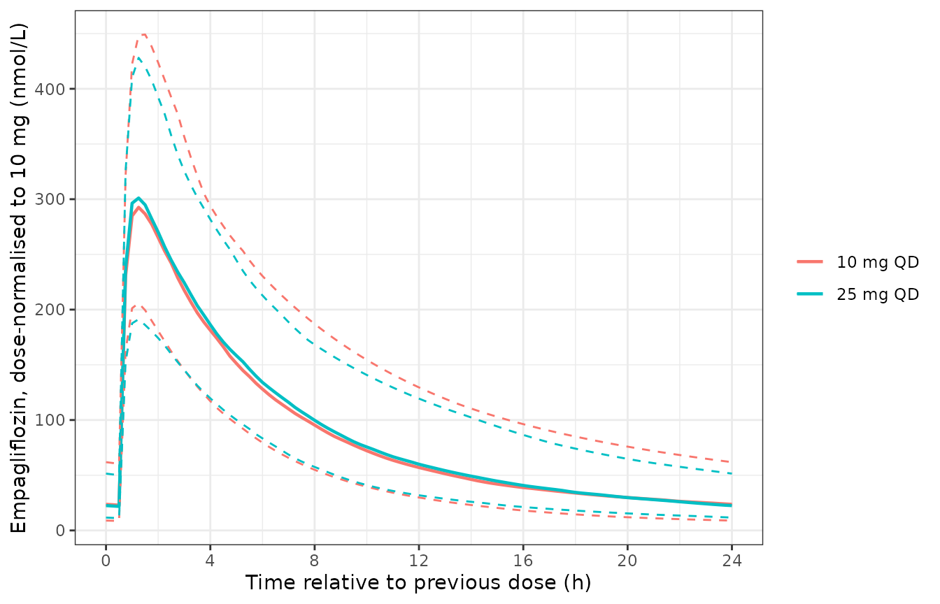

Replicates Figure 4 of Riggs 2013: median (solid) and 5th / 95th percentiles (dashed) of simulated dose-normalised empagliflozin concentrations over the final 24 h dosing interval at steady state.

dp <- vpc |>
  select(treatment, tad, p50) |>
  tidyr::pivot_wider(names_from = treatment, values_from = p50) |>
  mutate(pct_diff = 100 * (`25 mg QD` / `10 mg QD` - 1))

# Common random numbers across the two arms are NOT used here (each arm has its
# own subjects), so compare the population medians, which are robust.
summary(dp$pct_diff)
#>    Min. 1st Qu.  Median    Mean 3rd Qu.    Max. 
#>  -4.955   1.517   3.924   2.741   5.139   6.872
stopifnot(abs(median(dp$pct_diff)) < 10)

PKNCA validation

Non-compartmental analysis of the simulated steady-state interval, computed with PKNCA rather than an inline trapezoidal rule.

# rxSolve returns observation rows only (there is no evid column in its output),
# so the only filter needed is the mandatory !is.na(Cc).
sim_nca <- sim |>
  filter(!is.na(Cc)) |>
  select(id, time, Cc, treatment)

dose_df <- bind_rows(ev_10, ev_25) |>
  filter(evid == 1) |>
  select(id, time, amt, treatment) |>
  mutate(treatment = factor(treatment, levels = c("10 mg QD", "25 mg QD")))

conc_obj <- PKNCA::PKNCAconc(sim_nca, Cc ~ time | treatment + id,
                             concu = "nmol/L", timeu = "h")
dose_obj <- PKNCA::PKNCAdose(dose_df, amt ~ time | treatment + id,
                             doseu = "mg")

# Two intervals. Steady-state metrics come from the final dosing interval;
# half-life comes from the post-last-dose washout, because within a dosing
# interval the apparent slope is still contaminated by absorption (ka is only
# about four times beta here, so absorption is not complete at 24 h).
intervals <- data.frame(
  start     = c(ss_from,     ss_from + tau),
  end       = c(ss_from + tau, ss_from + tau + washout),
  cmax      = c(TRUE,  FALSE),
  tmax      = c(TRUE,  FALSE),
  cmin      = c(TRUE,  FALSE),
  auclast   = c(TRUE,  FALSE),
  cav       = c(TRUE,  FALSE),
  half.life = c(FALSE, TRUE)
)

nca <- PKNCA::pk.nca(PKNCA::PKNCAdata(conc_obj, dose_obj, intervals = intervals))
nca_res <- as.data.frame(nca)
head(nca_res)
#> # A tibble: 6 × 8
#>   treatment    id start   end PPTESTCD PPORRES exclude PPORRESU
#>   <fct>     <int> <dbl> <dbl> <chr>      <dbl> <chr>   <chr>   
#> 1 10 mg QD      1   648   672 auclast  1869.   <NA>    h*nmol/L
#> 2 10 mg QD      1   648   672 cmax      322.   <NA>    nmol/L  
#> 3 10 mg QD      1   648   672 cmin       14.3  <NA>    nmol/L  
#> 4 10 mg QD      1   648   672 tmax        1.25 <NA>    h       
#> 5 10 mg QD      1   648   672 cav        77.9  <NA>    nmol/L  
#> 6 10 mg QD      1   672   792 tmax        0    <NA>    h

Half-life versus each subject’s own analytic beta

The most informative NCA check here is not against a published summary but against the model’s own closed form: for each simulated subject, the terminal half-life PKNCA estimates must equal log(2)/beta computed from that subject’s own sampled cl, vc, vp and q. This is a per-subject identity, so a tight bound is correct.

subj_par <- sim |>
  group_by(id, treatment) |>
  summarise(cl = first(cl), vc = first(vc), vp = first(vp), q = first(q),
            .groups = "drop") |>
  mutate(
    k10  = cl / vc, k12 = q / vc, k21 = q / vp,
    bsum = k10 + k12 + k21,
    beta = (bsum - sqrt(bsum^2 - 4 * k10 * k21)) / 2,
    hl_analytic = log(2) / beta
  )

hl_cmp <- nca_res |>
  filter(start == ss_from + tau, PPTESTCD == "half.life") |>
  select(id, treatment, hl_nca = PPORRES) |>
  inner_join(subj_par, by = c("id", "treatment")) |>
  mutate(pct_diff = 100 * (hl_nca - hl_analytic) / hl_analytic)

stopifnot(nrow(hl_cmp) == 2L * n_per_arm)
summary(hl_cmp$pct_diff)
#>     Min.  1st Qu.   Median     Mean  3rd Qu.     Max. 
#> -0.73856 -0.23382 -0.13499 -0.17027 -0.06662 -0.00262

stopifnot(
  # Same drawn parameters on both sides: the residual is pure regression /
  # sampling-grid error, so assert on the centre AND on a robust quantile.
  abs(median(hl_cmp$pct_diff)) < 2,
  quantile(abs(hl_cmp$pct_diff), 0.9) < 5
)

Comparison against published non-compartmental values

Riggs 2013 does not tabulate its own NCA. Its Introduction does, however, summarise the observed non-compartmental behaviour of empagliflozin in this patient population, citing reference 10 (the Phase I study that became Study A): peak levels 1.5-3.0 h after dosing, mean terminal half-life 10-19 h, and up to 23% accumulation at steady state. Those are the only published NCA anchors available and they are reproduced below with that provenance made explicit.

published <- tibble::tribble(
  ~treatment,   ~half.life,
  "10 mg QD",   14.5,
  "25 mg QD",   14.5
)

# Each metric must be taken from the interval it belongs to. Requesting
# half.life on the washout interval makes PKNCA emit a companion `tmax` for that
# interval too (its value is 0, the interval start), so grouping on PPTESTCD
# alone would silently pool two different tmax populations. Select by interval
# start, then assert exactly one value per subject per metric so the mixing
# cannot come back unnoticed.
ss_metrics <- nca_res |>
  filter(start == ss_from, PPTESTCD %in% c("cmax", "tmax", "cav"))
hl_metrics <- nca_res |>
  filter(start == ss_from + tau, PPTESTCD == "half.life")

nca_long <- bind_rows(ss_metrics, hl_metrics)
stopifnot(
  # 2 arms x n_per_arm subjects x 1 value for each of cmax, tmax, cav, half.life
  nrow(nca_long) == 4L * 2L * n_per_arm,
  !any(duplicated(nca_long[c("treatment", "id", "PPTESTCD")]))
)

sim_summary <- nca_long |>
  group_by(treatment, PPTESTCD) |>
  summarise(PPORRES = median(PPORRES), .groups = "drop") |>
  tidyr::pivot_wider(names_from = PPTESTCD, values_from = PPORRES)

cmp <- nlmixr2lib::ncaComparisonTable(
  simulated     = sim_summary |> select(treatment, half.life),
  reference     = published,
  by            = "treatment",
  units         = c(half.life = "h"),
  tolerance_pct = 20
)
knitr::kable(
  cmp,
  caption = "Median simulated steady-state terminal half-life versus the midpoint of the 10-19 h observed range quoted in Riggs 2013 (Introduction, citing reference 10). * marks rows differing by >20%."
)

Median simulated steady-state terminal half-life versus the midpoint of the 10-19 h observed range quoted in Riggs 2013 (Introduction, citing reference 10). * marks rows differing by >20%.
NCA parameter	treatment	Reference	Simulated	% diff
t½ (h)	10 mg QD	14.5	13.7	-5.4%
t½ (h)	25 mg QD	14.5	13.5	-6.7%


knitr::kable(
  sim_summary |>
    dplyr::rename("Treatment" = treatment, "Cmax,ss (nmol/L)" = cmax,
                  "Tmax (h)" = tmax, "Cavg,ss (nmol/L)" = cav,
                  "t1/2 (h)" = half.life),
  digits = 2,
  caption = "Median simulated steady-state NCA parameters over the final 24 h dosing interval."
)

Median simulated steady-state NCA parameters over the final 24 h dosing interval.
Treatment	Cavg,ss (nmol/L)	Cmax,ss (nmol/L)	t1/2 (h)	Tmax (h)
10 mg QD	86.40	292.64	13.72	1.25
25 mg QD	224.17	767.44	13.53	1.25

tmax_med <- sim_summary$tmax
hl_med   <- sim_summary$half.life

stopifnot(
  # Terminal half-life falls inside the 10-19 h observed range quoted by the
  # paper. Median across the cohort, not an extreme.
  all(hl_med > 10 & hl_med < 19),
  # Tmax is a KNOWN deviation, so pin it rather than leave it unasserted: the
  # published model peaks around 1.25 h, below the 1.5-3.0 h observed range.
  # Asserting the band actually achieved makes this a regression test - if a
  # future edit moves Tmax into or far from the published range, this goes red.
  all(tmax_med > 1.0 & tmax_med < 1.5)
)

tmax_med
#> [1] 1.25 1.25

The simulated median Tmax (about 1.25 h) sits slightly earlier than the 1.5-3.0 h range quoted in the Introduction. This is an expected and documented consequence of the model the authors chose to publish, not a transcription error. Riggs 2013 Methods reports that a three-transit-compartment absorption model was required to fit the first few hours post-dose, but that it was abandoned for a simplified model with the absorption lag fixed at 0.5 h because the full covariate model ran “nearly 40 times faster” (about 45 minutes versus more than 29 hours), and that the fit was then restricted to observations collected after 1 hour post-dose. The published model is therefore not intended to reproduce the absorption peak, and the authors state explicitly that early observations “were not necessary for proper estimation of the included covariate effects”. The consequence is flagged here rather than tuned away.

Assumptions and deviations

Molecular weight is not from the paper. Riggs 2013 reports concentrations in nmol/L but never states a molecular weight. The model uses 450.91 g/mol (empagliflozin, BI 10773, CAS 864070-44-0, C23H27ClO7), which is the value already used by the sibling models Baron_2016_empagliflozin and Johnston_2021_empagliflozin_popPK. It is corroborated by the paper’s own numbers: it reproduces the published 25 mg AUCss triplet to better than 0.6% (see the primary validation above), which would not happen with a materially different value.
Minus signs recovered from the PDF byte stream. Four covariate exponents are printed with a minus sign that most PDF text extractors drop. They were recovered from the raw encoding and independently confirmed against the direction of the Figure 3 bootstrap densities; the check is reproduced in the “Recovering the dropped minus signs” section above.
SMK1 / SMK2 identification. Table 2 names the two smoking dummies only as SMK1 and SMK2. Figure 3A lists the matching categorical rows in the order “Ex-smoker”, “Current smoker”, “Consumes alcohol”, which is the same order as the Table 2 rows SMK1, SMK2, ALC – so SMK1 is the ex-smoker indicator and SMK2 the current-smoker indicator. Figure 3A’s per-row bootstrap percentages corroborate the pairing (the Ex-smoker row is majority below the null, matching 0.991; the Current smoker row is majority above it, matching 1.02). The distinction is in any case immaterial to predictions: both effects are within 1% of unity and the paper concludes smoking history does not affect PK.
Smoking reference category is reconstructed, not rebased. Riggs 2013 uses a never-smoker reference; the canonical SMOKE_NEVER / SMOKE_CURRENT pair uses a former-smoker reference. Rather than rebase the published multipliers (which would also require shifting the published base CL/F), the model derives the paper’s ex-smoker dummy in model() as 1 - SMOKE_NEVER - SMOKE_CURRENT. Every published number is therefore used exactly as printed.
Total protein and serum creatinine units. The Figure 3 caption states “total protein of 6.8 mg/dL, and serum creatinine of 0.8 g/dL”. Both unit strings are typographical errors: Table 1 reports total protein in g/dL (study means 6.62-7.42) and serum creatinine in mg/dL (study means 0.8-1.1), and the Figure 3A axis labels read “Total protein = 5.0 g/dL” and “SCr = 0.6 mg/dL”. The model uses total protein 6.8 g/dL (68 g/L in the canonical SI column) and serum creatinine 0.8 mg/dL.
New canonical covariate ALCOHOL_USE. The paper’s ALC covariate is any history of alcohol use (“Consumes alcohol” in Figure 3A, against a reference individual with “no history of alcohol use”). The register’s existing ALCOHOL_ABUSE entry denotes the much narrower chronic-abuse diagnosis, so a new canonical was registered rather than overloading it.
Study-group residual error. The two residual-error pairs are selected by the STUDY_DE covariate. It affects the residual error only; no structural or disposition parameter depends on it. Set STUDY_DE = 0 to reproduce the lower-variability Studies A/B/C behaviour.
Unreported cohort distributions. Riggs 2013 does not report the distribution of smoking status or alcohol history. The virtual cohort assumes 60% never / 25% former / 15% current smokers and 50% with any alcohol history. Neither assumption materially affects the simulations, because all three multipliers are within 2% of unity.
Absorption phase. As discussed above, the published model deliberately omits the transit-compartment absorption structure and was fitted only to observations after 1 h post-dose, so simulated Tmax runs slightly early relative to the observed 1.5-3.0 h range quoted in the paper’s Introduction. Use this model for exposure (AUC, Cavg, trough) rather than for peak timing.
No observed data. The figures use a virtual cohort approximating Riggs 2013 Table 1; the original patient-level data are not public.