Cefazolin (Wassef 2026)
Source:vignettes/articles/Wassef_2026_cefazolin.Rmd
Wassef_2026_cefazolin.RmdModel and source
- Citation: Wassef A, Kosicka-Noworzyn K, Back H, Siemiatkowska A, Yohn C, Sadek R, Kagan L, Brunetti L. Cefazolin surgical prophylaxis in obesity: a body composition-driven population pharmacokinetic approach. Antimicrob Agents Chemother. 2026. doi:10.1128/aac.01677-25. PMCID PMC13321816. Structural ODEs from Fig. 4b; all parameter estimates from Supplementary Table S2; covariates enter uncentred (see model()).
- Description: Two-compartment population PK model for intravenous bolus cefazolin surgical prophylaxis (2 g below 120 kg, 3 g at or above 120 kg) in adults undergoing sleeve gastrectomy or laparoscopic abdominal surgery, most with obesity (Wassef 2026, n = 87). Total plasma concentration plus a biophase (effect) compartment whose concentration times a partition coefficient gives the total subcutaneous adipose tissue concentration. Final covariates are bioimpedance (BIA) measured body composition: age and fat-free mass on CL, abdominal-trunk fat-free mass and trunk muscle mass on V1, total body water percentage on V2, body weight on ke0 and body fat percentage on the adipose partition coefficient. Log-normal IIV on all six parameters with a CL-V1 correlation; combined additive + proportional plasma error and additive tissue error. Estimated in Monolix 2024R1.
- Article: https://doi.org/10.1128/aac.01677-25 (open access, PMC13321816)
Wassef et al. fitted total plasma cefazolin and total subcutaneous
abdominal adipose tissue cefazolin jointly in Monolix 2024R1.
Disposition is a two-compartment model; adipose tissue is a massless
biophase (effect) compartment equilibrating with plasma at rate
ke0, and the measured tissue concentration is the biophase
concentration times a partition coefficient Kp. The final
covariates are body-composition measures from a Tanita MC-780 segmental
bioimpedance analyser.
Population
87 adults aged 18-65 years (46 women, 53%; 76% White) undergoing sleeve gastrectomy or laparoscopic abdominal hernia surgery at a single US centre (Table 1). Most had obesity: median weight 112.9 kg, median BMI 38 kg/m^2, 36 of 87 with BMI >= 40 and 70 of 87 with an unhealthy body-fat percentage (Table 1, Supplementary Table S1). Patients under 120 kg received a 2 g intravenous bolus (n = 57); those at or above 120 kg received 3 g (n = 30), re-dosed every 4 h during surgery (two subjects received a second dose). Plasma was sampled at 5, 30, 60, 120 and 240 min after the dose and adipose tissue was biopsied at incision and at closure.
The same information is available programmatically via
readModelDb("Wassef_2026_cefazolin")()$population.
Source trace
| Equation / parameter | Value | Source location |
|---|---|---|
d/dt(central), d/dt(peripheral1)
|
n/a | Fig. 4b equations (1)-(2) |
d/dt(effect) <- ke0 * (central / vc - effect) |
n/a | Fig. 4b equation (3) |
Cc <- central / vc |
n/a | Fig. 4b equation (4) |
Cadipose <- kp_adipose * effect |
n/a | Fig. 4b equation (5) |
lcl |
log(3.9 L/h) | Table S2 CLpop
|
lvc |
log(3.6 L) | Table S2 V1pop
|
lq |
log(11 L/h) | Table S2 Qpop
|
lvp |
log(1.1 L) | Table S2 V2pop
|
lke0 |
log(1.91 1/h) | Table S2 ke0pop
|
lkp_adipose |
log(0.37) | Table S2 Kppop
|
e_age_cl |
-0.011 /year | Table S2 beta CL-AGE
|
e_ffm_cl |
0.0052 /kg | Table S2 beta CL-FFMAMT
|
e_ffm_trunk_vc |
-0.64 /kg | Table S2 beta V1-MBDFFMAMT
|
e_muscle_mass_trunk_vc |
0.69 /kg | Table S2 beta V1-MBDMSLAMT
|
e_bodywater_pct_vp |
0.033 /% | Table S2 beta V2-WTRPER
|
e_wt_ke0 |
0.025 /kg | Table S2 beta ke0-WTKG
|
e_bodyfat_pct_kp_adipose |
-0.063 /% | Table S2 beta Kp-FATPER
|
etalcl + etalvc |
0.27^2, 0.59 x 0.27 x 0.25, 0.25^2 | Table S2 Omega CL, Omega V1, corr(V1, CL) |
etalq, etalvp
|
0.41^2, 0.33^2 | Table S2 Omega Q, Omega V2 |
etalke0, etalkp_adipose
|
0.68^2, 0.51^2 | Table S2 Omega ke0, Omega Kp |
addSd, propSd
|
51.4 mg/L, 0.095 | Table S2 plasma combined 2 error |
addSd_Cadipose |
6.1 mg/L | Table S2 tissue constant error |
Covariates enter uncentred, P = Ppop * exp(beta * COV),
so each Ppop is the value at covariate 0; the section
Covariate centring below gives the evidence.
Virtual cohort
The subject-level data are not public. Each dose arm gets 200 virtual
subjects drawn from the Table S1 dose-group means and SDs. These moments
already describe each arm’s weight range, so weight is bounded only to a
physiological 45-250 kg rather than at the 120 kg dose-assignment
threshold. Bioimpedance fat-free mass is weight minus fat mass, so
FFM is derived from weight and body-fat percentage. The
trunk and water measures are then scaled from FFM with the
Table S1 cohort-mean ratios: trunk fat-free mass = 0.545 x
FFM (37.33 / 68.47 kg); trunk muscle = trunk fat-free mass
minus the arm’s Table S1 mean gap (1.57 kg for 2 g, 1.80 kg for 3 g);
body water = 0.7145 x FFM (48.92 / 68.47 kg). Deriving them
rather than drawing them independently matters. V1 depends on
exp(0.69 * MUSCLE_MASS_TRUNK - 0.64 * FFM_TRUNK), and every
1 kg of independent noise in the gap between the two trunk measures
would halve or double V1.
# set.seed() fixes the covariate draws; rxSetSeed() fixes rxode2's IIV draws
# for a given solver thread count only, so every assertion below is written to
# hold for any cohort the model can produce.
set.seed(20260529)
rxode2::rxSetSeed(20260529)

rtnorm <- function(n, mean, sd, lo, hi) {
  stats::qnorm(stats::runif(n, stats::pnorm(lo, mean, sd), stats::pnorm(hi, mean, sd)), mean, sd)
}

make_arm <- function(n, dose_mg, wt, fat, age, trunk_gap, id_offset) {
  WT <- rtnorm(n, wt[1], wt[2], 45, 250)
  BODYFAT_PCT <- rtnorm(n, fat[1], fat[2], 15, 60)
  FFM <- WT * (1 - BODYFAT_PCT / 100)
  FFM_TRUNK <- FFM * 37.33 / 68.47
  tibble(
    id = id_offset + seq_len(n),
    dose_mg = dose_mg,
    arm = paste(dose_mg / 1000, "g"),
    WT = WT,
    BODYFAT_PCT = BODYFAT_PCT,
    FFM = FFM,
    FFM_TRUNK = FFM_TRUNK,
    MUSCLE_MASS_TRUNK = FFM_TRUNK - trunk_gap,
    BODYWATER_PCT = 100 * 0.7145 * FFM / WT,
    AGE = rtnorm(n, age[1], age[2], 18, 65)
  )
}

# Table S1 dose-group mean (SD): weight, FATPER; Table 1: age. Trunk gap =
# mean(MBDFFMAMT) - mean(MBDMSLAMT) per arm, Table S1.
cohort <- bind_rows(
  make_arm(200, 2000, wt = c(95.4, 18.3), fat = c(34.9, 10.33), age = c(49, 13.4),
           trunk_gap = 34.39 - 32.82, id_offset = 0L),
  make_arm(200, 3000, wt = c(146.9, 24.6), fat = c(43.6, 6.43), age = c(41, 14.6),
           trunk_gap = 42.98 - 41.18, id_offset = 200L)
)
stopifnot(!anyDuplicated(cohort$id))

cohort |>
  group_by(arm) |>
  summarise(across(c(WT, BODYFAT_PCT, FFM, FFM_TRUNK, MUSCLE_MASS_TRUNK, BODYWATER_PCT, AGE),
                   ~ round(median(.x), 1))) |>
knitr::kable(caption = "Virtual cohort medians by arm (Table S1 medians: 2 g weight 98.6 kg, FATPER 35.2%, FFMAMT 62.8 kg, MBDFFMAMT 34.3 kg, MBDMSLAMT 32.7 kg, WTRPER 45.3%; 3 g 142.9 kg, 44.5%, 78 kg, 43.1 kg, 41.2 kg, 40.2%).")| arm | WT | BODYFAT_PCT | FFM | FFM_TRUNK | MUSCLE_MASS_TRUNK | BODYWATER_PCT | AGE |
|---|---|---|---|---|---|---|---|
| 2 g | 94.2 | 35.0 | 62.4 | 34.0 | 32.5 | 46.4 | 47.2 |
| 3 g | 150.2 | 43.7 | 84.2 | 45.9 | 44.1 | 40.3 | 42.2 |
Simulation
The event table doses central and observes on a fine 0-4
h grid that also contains the paper’s sampling times and the incision
and closure biopsy times. The model has two endpoints (Cc,
Cadipose), so observation rows carry dvid = 1.
rxode2 returns both concentrations on every row.
t_incision <- 0.06 # h; median incision biopsy time read from Fig. 3
t_closure <- 0.6   # h; median closure biopsy time read from Fig. 3
t_paper <- round(c(5 / 60, 0.5, 1, 2, 4), 6) # rounded like t_obs so %in% matches
t_obs <- sort(unique(round(c(0, seq(0.02, 4, by = 0.02), t_paper, t_incision, t_closure), 6)))

make_events <- function(cov) {
  dose <- cov |> mutate(time = 0, amt = dose_mg, evid = 1L, cmt = "central", dvid = NA_integer_)
  obs <- cov |>
    select(-dose_mg) |>
    tidyr::crossing(time = t_obs) |>
    mutate(amt = 0, evid = 0L, cmt = NA_character_, dvid = 1L)
  bind_rows(dose |> select(-dose_mg), obs) |>
    arrange(id, time, desc(evid))
}
events <- make_events(cohort)

mod <- readModelDb("Wassef_2026_cefazolin")
sim <- rxode2::rxSolve(mod, events = events, keep = c("arm", "BODYFAT_PCT")) |>
  as.data.frame()
#> ℹ parameter labels from comments will be replaced by 'label()'
Replicate published figures
# Replicates Figure 2 of Wassef 2026: total plasma cefazolin, 0-4 h, by dose.
sim |>
  filter(time > 0) |>
  group_by(arm, time) |>
  summarise(Q05 = quantile(Cc, 0.05), Q50 = median(Cc), Q95 = quantile(Cc, 0.95),
            .groups = "drop") |>
  ggplot(aes(time, Q50)) +
  geom_ribbon(aes(ymin = Q05, ymax = Q95), alpha = 0.25) +
  geom_line() +
  facet_wrap(~arm) +
  scale_y_log10() +
  labs(x = "Time after dose (h)", y = "Total plasma cefazolin (mg/L)",
       title = "Plasma cefazolin: median and 90% interval",
       caption = "Replicates Figure 2 of Wassef 2026.")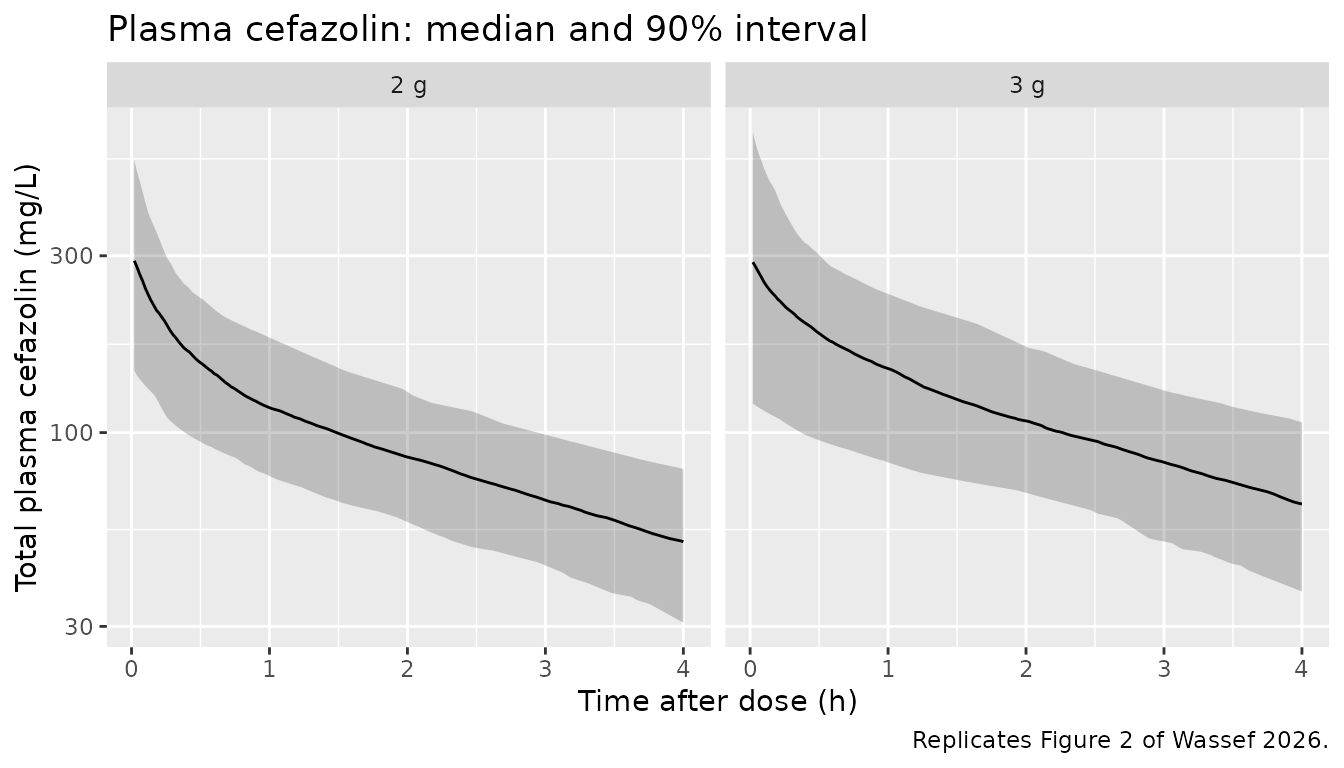
# Replicates Figure 3 of Wassef 2026: subcutaneous adipose cefazolin against
# the 4 / 8 / 16 ug/mL MIC lines, split at the median body-fat percentage.
sim |>
  filter(time > 0) |>
  mutate(fat_group = ifelse(BODYFAT_PCT < median(cohort$BODYFAT_PCT),
                            "Body fat below cohort median", "Body fat above cohort median")) |>
  group_by(fat_group, time) |>
  summarise(Q05 = quantile(Cadipose, 0.05), Q50 = median(Cadipose),
            Q95 = quantile(Cadipose, 0.95), .groups = "drop") |>
  ggplot(aes(time, Q50)) +
  geom_ribbon(aes(ymin = Q05, ymax = Q95), alpha = 0.25) +
  geom_line() +
  geom_hline(yintercept = c(4, 8, 16), linetype = "dashed") +
  facet_wrap(~fat_group) +
  coord_cartesian(ylim = c(0, 40)) +
  labs(x = "Time after dose (h)", y = "Adipose cefazolin (mg/L)",
       title = "Subcutaneous adipose cefazolin: median and 90% interval",
       caption = "Replicates Figure 3 of Wassef 2026 (observed points range 0-39 ug/mL).")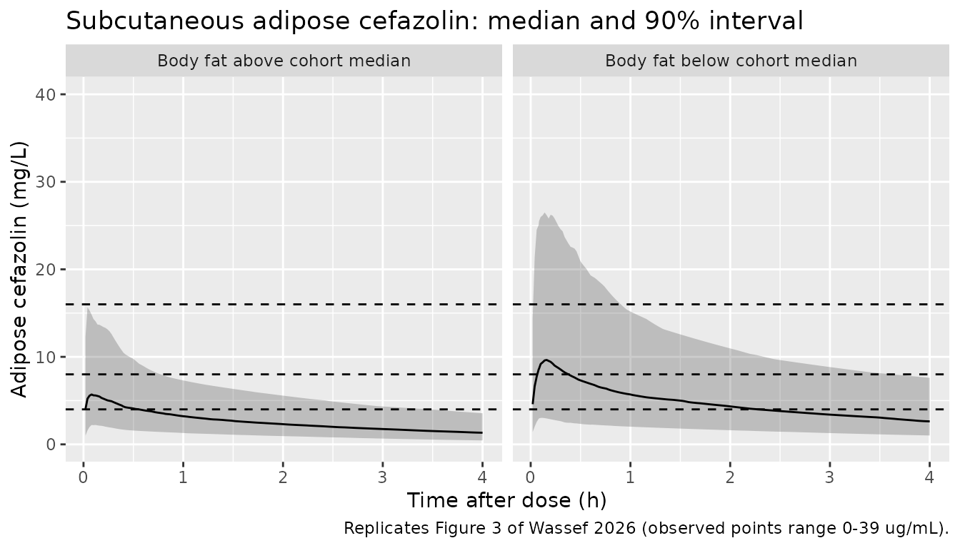
Adipose target attainment (Table 3)
Table 3 reports the observed share of patients whose adipose concentration was above 16, 8 and 4 ug/mL at incision and at closure. It also reports the share above each threshold at both biopsies, for the whole duration of surgery. These are observed counts from 87 patients, so each percentage carries a binomial standard error of about 5 percentage points.
attain <- function(d) {
  c(`>16` = 100 * mean(d > 16), `>8` = 100 * mean(d > 8), `>4` = 100 * mean(d > 4))
}
at_inc <- sim |> filter(abs(time - t_incision) < 1e-6) |> arrange(id)
at_clo <- sim |> filter(abs(time - t_closure) < 1e-6) |> arrange(id)
stopifnot(nrow(at_inc) == nrow(cohort), nrow(at_clo) == nrow(cohort),
          identical(at_inc$id, at_clo$id))
both <- pmin(at_inc$Cadipose, at_clo$Cadipose)

tab3 <- tibble(
  Timepoint = rep(c("Incision", "Closure", "Duration of surgery"), each = 3),
  MIC = rep(c(">16", ">8", ">4"), 3),
  Published = c(12.6, 34.6, 54, 6.9, 33.3, 66.6, 3.4, 17.2, 40.2),
  Simulated = round(c(attain(at_inc$Cadipose), attain(at_clo$Cadipose), attain(both)), 1)
) |>
  mutate(Difference = Simulated - Published)
tab3 |>
  rename("MIC (ug/mL)" = MIC, "Published (%)" = Published, "Simulated (%)" = Simulated,
         "Difference (points)" = Difference) |>
knitr::kable(caption = "Share of patients above each MIC in adipose tissue, all patients (Table 3).")| Timepoint | MIC (ug/mL) | Published (%) | Simulated (%) | Difference (points) |
|---|---|---|---|---|
| Incision | >16 | 12.6 | 9.8 | -2.8 |
| Incision | >8 | 34.6 | 37.0 | 2.4 |
| Incision | >4 | 54.0 | 76.5 | 22.5 |
| Closure | >16 | 6.9 | 5.2 | -1.7 |
| Closure | >8 | 33.3 | 25.8 | -7.5 |
| Closure | >4 | 66.6 | 64.2 | -2.4 |
| Duration of surgery | >16 | 3.4 | 4.2 | 0.8 |
| Duration of surgery | >8 | 17.2 | 21.0 | 3.8 |
| Duration of surgery | >4 | 40.2 | 62.3 | 22.1 |
# Each published cell carries ~5 points of binomial error and the simulated
# cohort ~2.5 more. The median-centred reading of the same estimates puts
# 68-100% of subjects above every threshold (see 'Covariate centring'), up to
# ~90 points off, so both bounds still fail on a wrong covariate centre.
# Realised max 18.8-22.5 and median 2.8-6.8 points over four seeds.
stopifnot(median(abs(tab3$Difference)) < 12, max(abs(tab3$Difference)) < 30)
Seven of the nine cells fall within about 8 points of the observed share. The model over-predicts attainment of the lowest threshold, 4 ug/mL, at incision and across the whole surgery by about 20 points. The single nominal incision time (0.06 h) is one candidate; Table 3 counts are also from only 87 patients.
PKNCA validation
NCA uses the paper’s own plasma sampling design (0, 5, 30, 60, 120,
240 min) on the individual predictions (Cc, no residual
error). Table 2 reports arithmetic means, so the simulated summary below
is also the mean across subjects.
sim_nca <- sim |>
  filter(!is.na(Cc)) |>
  semi_join(tibble(time = c(0, t_paper)), by = "time") |>
  select(id, time, Cc, arm)
sim_nca <- bind_rows(
  sim_nca,
  sim_nca |> distinct(id, arm) |> mutate(time = 0, Cc = 0)
) |>
  distinct(id, arm, time, .keep_all = TRUE) |>
  arrange(id, arm, time)

conc_obj <- PKNCA::PKNCAconc(sim_nca, Cc ~ time | arm + id)
dose_df <- events |> filter(evid == 1) |> select(id, time, amt, arm)
dose_obj <- PKNCA::PKNCAdose(dose_df, amt ~ time | arm + id, route = "intravascular")

intervals <- data.frame(start = 0, end = Inf, aucinf.obs = TRUE, cl.obs = TRUE,
                        half.life = TRUE, vss.obs = TRUE)
nca_res <- PKNCA::pk.nca(PKNCA::PKNCAdata(conc_obj, dose_obj, intervals = intervals))

sim_mean <- as.data.frame(nca_res) |>
  filter(PPTESTCD %in% c("aucinf.obs", "cl.obs", "half.life", "vss.obs")) |>
  group_by(arm, PPTESTCD) |>
  summarise(PPORRES = mean(PPORRES, na.rm = TRUE), .groups = "drop") |>
  tidyr::pivot_wider(names_from = PPTESTCD, values_from = PPORRES)
Comparison against published NCA
# Table 2 means; AUC0-inf printed in h*g/L (0.72, 0.80) converted to mg*h/L.
published <- tibble::tribble(
  ~arm,  ~aucinf.obs, ~cl.obs, ~half.life, ~vss.obs,
  "2 g", 720,         3.2,     2.66,       10.3,
  "3 g", 800,         4.35,    2.44,       12.7
)

cmp <- nlmixr2lib::ncaComparisonTable(
  simulated = sim_mean,
  reference = published,
  by = "arm",
  units = c(aucinf.obs = "mg*h/L", cl.obs = "L/h", half.life = "h", vss.obs = "L"),
  tolerance_pct = 20
)
knitr::kable(cmp, caption = "Simulated (mean) vs. Table 2 NCA (mean). * differs by >20%.")| NCA parameter | arm | Reference | Simulated | % diff |
|---|---|---|---|---|
| AUC0-∞ (obs) (mg*h/L) | 2 g | 720 | 636 | -11.7% |
| AUC0-∞ (obs) (mg*h/L) | 3 g | 800 | 815 | +1.9% |
| t½ (h) | 2 g | 2.66 | 2.69 | +1.1% |
| t½ (h) | 3 g | 2.44 | 2.88 | +18.1% |
| CL/F (L/h) | 2 g | 3.2 | 3.4 | +6.3% |
| CL/F (L/h) | 3 g | 4.35 | 4.03 | -7.4% |
| Vss/F (L) | 2 g | 10.3 | 12.1 | +17.1% |
| Vss/F (L) | 3 g | 12.7 | 15.9 | +25.2%* |
cmp_num <- sim_mean |>
  tidyr::pivot_longer(-arm, names_to = "param", values_to = "sim") |>
  inner_join(tidyr::pivot_longer(published, -arm, names_to = "param", values_to = "pub"),
             by = c("arm", "param")) |>
  mutate(pct = 100 * (sim - pub) / pub)
stopifnot(nrow(cmp_num) == 8L)
# Structural: CL and AUC move together with any mis-transcribed CL, V or
# covariate centre by tens of percent. Realised max 8.7-11.7% over four seeds.
stopifnot(all(abs(cmp_num$pct[cmp_num$param %in% c("aucinf.obs", "cl.obs")]) < 20))
AUC0-inf and CL agree with Table 2 within about 12% in both arms, and
the 2 g half-life within a few percent. Vss runs high, by about 17% in
the 2 g arm and 25% in the 3 g arm, and the 3 g half-life by about 18%.
Those quantities depend on V1 and V2, which in this model hang on the
trunk and body-water measures that the virtual cohort can only
approximate (see Virtual cohort). The comparison helper labels
clearance and Vss CL/F and Vss/F; the dose
here is intravenous, so they are CL and Vss.
Covariate centring
The Methods state that continuous covariates “were centered on their
median values”, and the display equations print
P = Ppop * (COV / COVmed)^beta. The fitted coefficients
rule out the power form. Under it, every coefficient except the two on
V1 changes its parameter by less than 8% across the whole cohort;
Kp, for example, would move only from 0.39 to 0.36 over
18-58% body fat. That cannot produce the 2- to 8.5-fold differences in
adipose target attainment of Table 3. The coefficients are slopes of an
exponential, exp(beta * COV), and the remaining question is
whether COV is centred on its median. The chunk below
re-solves the model with each covariate centred on its Table S1 median
and compares typical-value predictions, all subjects at their own
covariates with no IIV.
mod_centred <- rxode2::rxode(mod) |>
  rxode2::model(cl <- exp(lcl + etalcl + e_age_cl * (AGE - 46) + e_ffm_cl * (FFM - 65))) |>
  rxode2::model(vc <- exp(lvc + etalvc + e_ffm_trunk_vc * (FFM_TRUNK - 37.1) +
                            e_muscle_mass_trunk_vc * (MUSCLE_MASS_TRUNK - 35.4))) |>
  rxode2::model(vp <- exp(lvp + etalvp + e_bodywater_pct_vp * (BODYWATER_PCT - 42.7))) |>
  rxode2::model(ke0 <- exp(lke0 + etalke0 + e_wt_ke0 * (WT - 112.9))) |>
  rxode2::model(kp_adipose <- exp(lkp_adipose + etalkp_adipose +
                                    e_bodyfat_pct_kp_adipose * (BODYFAT_PCT - 40.2)))
#> ℹ parameter labels from comments will be replaced by 'label()'

typ <- function(m, label) {
  s <- rxode2::rxSolve(rxode2::zeroRe(m), events = events, keep = "arm") |> as.data.frame()
  plasma <- s |>
    filter(arm == "2 g", time %in% t_paper) |>
    group_by(time) |>
    summarise(v = median(Cc), .groups = "drop")
  inc <- s |> filter(abs(time - t_incision) < 1e-6)
  clo <- s |> filter(abs(time - t_closure) < 1e-6)
  tibble(
    Reading = label,
    `2 g plasma at 5 min / 0.5 / 1 / 2 / 4 h (mg/L)` = paste(round(plasma$v), collapse = " / "),
    `Adipose at incision, median (mg/L)` = round(median(inc$Cadipose), 1),
    `Adipose at closure, median (mg/L)` = round(median(clo$Cadipose), 1),
    `Closure >4 ug/mL (%)` = round(100 * mean(clo$Cadipose > 4))
  )
}
centring <- bind_rows(
  tibble(Reading = "Published (Fig. 2, Fig. 3, Table 3)",
         `2 g plasma at 5 min / 0.5 / 1 / 2 / 4 h (mg/L)` = "~250-400 / 150-250 / 100-200 / 70-130 / 30-70",
         `Adipose at incision, median (mg/L)` = NA, `Adipose at closure, median (mg/L)` = NA,
         `Closure >4 ug/mL (%)` = 66.6),
  typ(mod, "Uncentred (packaged model)"),
  typ(mod_centred, "Centred on Table S1 medians")
)
#> ℹ parameter labels from comments will be replaced by 'label()'
#> ℹ omega/sigma items treated as zero: 'etalcl', 'etalvc', 'etalq', 'etalvp', 'etalke0', 'etalkp_adipose'
#> Warning: multi-subject simulation without without 'omega'
#> ℹ omega/sigma items treated as zero: 'etalcl', 'etalvc', 'etalq', 'etalvp', 'etalke0', 'etalkp_adipose'
#> Warning: multi-subject simulation without without 'omega'
knitr::kable(centring, caption = "Typical-value predictions under the two readings. Fig. 2 and Fig. 3 ranges were read by eye; Fig. 3 adipose points mostly lie between 1 and 15 ug/mL.")| Reading | 2 g plasma at 5 min / 0.5 / 1 / 2 / 4 h (mg/L) | Adipose at incision, median (mg/L) | Adipose at closure, median (mg/L) | Closure >4 ug/mL (%) |
|---|---|---|---|---|
| Published (Fig. 2, Fig. 3, Table 3) | ~250-400 / 150-250 / 100-200 / 70-130 / 30-70 | NA | NA | 66.6 |
| Uncentred (packaged model) | 253 / 150 / 116 / 88 / 53 | 7 | 4.9 | 68.0 |
| Centred on Table S1 medians | 442 / 267 / 179 / 81 / 17 | 29 | 88.7 | 100.0 |
# The centred reading puts every closure biopsy above 4 ug/mL (Table 3: 66.6%);
# the uncentred one does not. A 15-fold gap, not a noise-level one.
stopifnot(centring$`Closure >4 ug/mL (%)`[3] > 95, centring$`Closure >4 ug/mL (%)`[2] < 90)
Read uncentred, the estimates give at the cohort medians
Kp of about 0.03 and ke0 of about 32 /h.
Adipose tissue therefore tracks plasma almost instantly at about 3% of
its concentration, which is the flat pattern of Fig. 3. The same reading
reproduces Fig. 2, the Table 2 NCA and Table 3 (above). Centred, the
model overshoots adipose concentrations about 15-fold and gives a plasma
half-life near 1 h against the NCA’s 2.6 h. The packaged model is
therefore uncentred, and lcl, lvc,
lvp, lke0 and lkp_adipose are
values at covariate 0 with no clinical meaning on their own. This is
what Monolix reports when a covariate enters untransformed.
Assumptions and deviations
-
Uncentred covariates. The model uses
P = Ppop * exp(beta * COV), contrary to the Methods sentence on median centring and to the printed power equations. The section above gives the evidence. With centring gone, the two values needed only for centring no longer matter: the unreported age median, and the Table S1 trunk-muscle median of 25.4 kg, which lies outside both dose-group medians (32.7 and 41.2 kg) and is a misprint. - Q and V2 as printed (11 L/h and 1.1 L). The maintainers checked the reading with the two values swapped. It fits Fig. 2 worse, and Table S2’s SE, RSE and bootstrap columns all agree with the printed order.
-
IIV is log-normal for all six parameters. The
Results describe the CL, V1 and V2 random effects as normally
distributed, but Table S2’s C.V. column equals
sqrt(exp(omega^2) - 1)on every row (0.27 gives 26.98%), which holds only for a log-normal SD. The CL-V1 covariance is 0.59 x 0.27 x 0.25. - Tissue residual error is additive. The Results call it a constant error with a lognormal distribution, but Table S2 prints it as 6.1 ug/mL; read as a log-scale SD it would imply a several-hundred-fold residual.
-
Plasma residual error is Monolix
combined 2,sqrt(a^2 + (b * f)^2), encoded withcombined2(). -
Sign of the weight effect on ke0. The Discussion
says ke0 decreased with body weight, but Table S2 gives
beta ke0-WTKG = +0.025with a wholly positive bootstrap interval (0.0087-0.045). The printed estimate is used. -
Fat-free mass is measured, not formula-based.
FFMis the Tanita bioimpedance fat-free mass (source columnFFMAMT). - Tissue units. Adipose concentrations were assayed in ug/g. They are reported in mg/L assuming a tissue density of 1 g/mL.
-
Virtual cohort. Weight, body fat and age are drawn
independently within each arm from Table S1 / Table 1 summaries. The
trunk and water measures are derived from
FFMwith cohort-mean ratios (see Virtual cohort). Sex, height and BMI do not enter the model and are not simulated. - Biopsy times. Incision (0.06 h) and closure (0.6 h) are the medians read by the maintainers from Fig. 3. A minority of closure biopsies fell between 1.5 and 4.3 h; they are not represented.
- Comparators. Table 2 and Table 3 summarise observed data from 85-87 patients and are compared with model simulations, not with simulations reported by the authors.
- No erratum or correction notice was found as of 2026-10-17.