Isoniazid, rifampicin, pyrazinamide and ethambutol PK and sputum bacillary load (Kloprogge 2020)
Source:vignettes/articles/Kloprogge_2020_tuberculosis.Rmd
Kloprogge_2020_tuberculosis.RmdModel and source
Kloprogge et al. (2020) analysed a longitudinal cohort of Malawian adults with drug-sensitive pulmonary tuberculosis on standard first-line therapy. They fitted one population PK model per first-line drug to steady-state plasma concentrations and a population PKPD model to serial sputum colony counts. The PKPD model takes the individual steady-state isoniazid and rifampicin AUC0-24 from the PK models as covariates. The paper contributes five model files:
| Model | Content |
|---|---|
Kloprogge_2020_isoniazid |
2-compartment PK, first-order absorption |
Kloprogge_2020_rifampicin |
1-compartment PK, Savic transit absorption |
Kloprogge_2020_pyrazinamide |
1-compartment PK, first-order absorption |
Kloprogge_2020_ethambutol |
2-compartment PK, one transit compartment |
Kloprogge_2020_hrze_bacterialload |
Biphasic sputum CFU decline with PK-exposure covariates |
- Citation: Kloprogge F, Mwandumba HC, Banda G, Kamdolozi M, Shani D, Corbett EL, Kontogianni N, Ward S, Khoo SH, Davies GR, Sloan DJ. (2020). Longitudinal pharmacokinetic-pharmacodynamic biomarkers correlate with treatment outcome in drug-sensitive pulmonary tuberculosis: a population pharmacokinetic-pharmacodynamic analysis. Open Forum Infect Dis 7(7):ofaa218. doi:10.1093/ofid/ofaa218.
- Article: https://doi.org/10.1093/ofid/ofaa218 (open access; PMC7378673). The structural equations and all parameter estimates are in the Supplementary Materials (S1 Table for PK, S2 Table for PKPD).
Population
Adults aged 16-65 years with smear-positive pulmonary tuberculosis were recruited at Queen Elizabeth Central Hospital, Blantyre, Malawi (Table 1). They received daily fixed-dose-combination tablets by weight band: in the intensive phase each RZHE tablet contained rifampicin 150 mg, isoniazid 75 mg, pyrazinamide 400 mg and ethambutol 275 mg, with 2 tablets at 30-37 kg, 3 at 37-54 kg, 4 at 54-74 kg and 5 above 74 kg. Plasma samples were taken on day 14 or 21, predose and 2 and 6 h after an observed fasted dose. Sputum was collected on days 0, 2, 4, 7, 14, 28, 49 and 56 for serial sputum colony counting (SSCC).
- PK cohort: 154 patients; median age 30 years (17-61); median weight 52 kg (34-74); 69% male; 58% HIV-positive.
- PKPD cohort: the 102 patients with at least two bacterial-load samples; median weight 53 kg (35-74); 74% male; 32% reported alcohol consumption; median baseline bilirubin 7.5 umol/L (1-32).
Source trace
| Item | Value | Source |
|---|---|---|
| Isoniazid CL/F, Vc/F (63 kg) | 13.70 L/h, 39.7 L | S1 Table |
| Isoniazid Q/F, Vp/F, ka | 2.9 L/h, 16.5 L, 0.6 1/h (held constant) | S1 Table; values from Seng 2015 |
| Isoniazid IIV CL, ka | 46.66%, 36.64% CV (ka held constant) | S1 Table |
| Isoniazid proportional error | 21.10% | S1 Table |
| Rifampicin CL/F, V/F (70 kg) | 16.90 L/h, 31.3 L | S1 Table |
| Rifampicin ka, MTT, NN | 0.277 1/h, 0.326 h, 1.5 (held constant) | S1 Table; values from Sloan 2017 |
| Rifampicin male effect on CL/F | 0.183 (log scale) | S1 Table ‘Cl~Male’ |
| Rifampicin IIV CL, V, MTT | 40.08%, 84.52%, 27.05% CV (MTT held constant) | S1 Table |
| Rifampicin proportional error | 19.40% | S1 Table |
| Pyrazinamide CL/F, V/F (70 kg) | 3.86 L/h, 45.2 L | S1 Table |
| Pyrazinamide ka | 3.94 1/h (held constant) | S1 Table; value from Alsultan 2017 |
| Pyrazinamide IIV CL, V, ka | 28.60%, 3.95%, 397.2% CV | S1 Table |
| Pyrazinamide residual error | 3.06% proportional; additive 74.5 (umol/L)^2 | S1 Table (see Assumptions) |
| Ethambutol CL/F, Vc/F (50 kg) | 45.50 L/h, 124.0 L | S1 Table |
| Ethambutol Q/F, Vp/F, ka, MTT | 34.3 L/h, 623 L, 0.474 1/h, 0.789 h (held constant) | S1 Table; values from Jonsson 2011 |
| Ethambutol IIV CL, ka, MTT | 20.99%, 67.56%, 109.6% CV (ka, MTT held constant) | S1 Table |
| Ethambutol proportional error | 12.80% | S1 Table |
| Allometric scaling, reference weights | CL x (WT/ref)^0.75, V x (WT/ref); 63, 70, 70, 50 kg | Supplementary section 2 |
| IIV convention | CV = 100 x sqrt(exp(omega^2) - 1) | S1 Table footnote |
| PKPD ODE | dB/dt = -knet B, knet = LAM (1 - BETA (1 - exp(-t ln2 / T1/2))) | Supplementary section 4 |
| Baseline load BL | 6.3867 log10 CFU/mL, additive IIV | S2 Table |
| LAM, T1/2, BETA | 0.0389 1/h, 149.58 h, 0.6445 | S2 Table |
| Isoniazid AUC0-24 on LAM | exp(0.0005 (AUC - 137.3)), AUC in umol*h/L | S2 Table; Figure 4 caption (units) |
| Baseline bilirubin on LAM | exp(0.0029 (TBILI - 7.5)) | S2 Table; Table 1 (median) |
| Alcohol on LAM | 1 - 0.0377 | S2 Table; Supplementary section 4 (form) |
| Rifampicin AUC0-24 on T1/2 | exp(0.0335 (AUC - 35.36)), AUC in umol*h/L | S2 Table |
| IIV block (BL, LAM, T1/2, BETA) | 4 x 4 variance-covariance | S2 Table |
| Residual error | variance 2.5832 on log10 CFU/mL (SD 1.607) | S2 Table ‘RUV’ |
Pharmacokinetics
Virtual cohort
The weight distribution matches Table 1 (median 52 kg, range 34-74 kg) and 31% of the cohort are female. Doses follow the weight bands. Each patient takes a daily dose for 14 days, and the 24-hour interval after the day-14 dose is analysed as steady state.
set.seed(20200703)
rxode2::rxSetSeed(20200703)

n_pk <- 154
cohort <- tibble(
  id = seq_len(n_pk),
  WT = pmin(pmax(round(exp(rnorm(n_pk, log(52), 0.15)), 1), 34), 74),
  SEXF = rbinom(n_pk, 1, 0.31)
) |>
  mutate(tablets = case_when(WT < 37 ~ 2, WT < 54 ~ 3, WT <= 74 ~ 4, TRUE ~ 5))

drugs <- tibble(
  drug = c("isoniazid", "rifampicin", "pyrazinamide", "ethambutol"),
  model = paste0("Kloprogge_2020_", c("isoniazid", "rifampicin", "pyrazinamide", "ethambutol")),
  mg_per_tablet = c(75, 150, 400, 275),
  dose_cmt = c("depot", "depot", "depot", "transit1"),
  mw = c(137.14, 822.94, 123.11, 204.31)
)

t_last_dose <- 13 * 24
obs_times <- t_last_dose + sort(unique(c(seq(0, 8, by = 0.25), seq(8.5, 24, by = 0.5))))

make_pk_events <- function(drug_row) {
  doses <- cohort |>
    tidyr::crossing(time = seq(0, t_last_dose, by = 24)) |>
    mutate(amt = tablets * drug_row$mg_per_tablet, evid = 1L, cmt = drug_row$dose_cmt)
  obs <- cohort |>
    tidyr::crossing(time = obs_times) |>
    mutate(amt = NA_real_, evid = 0L, cmt = "central")
  bind_rows(doses, obs) |>
    arrange(id, time, desc(evid))
}

sim_pk <- lapply(seq_len(nrow(drugs)), function(i) {
  ev <- make_pk_events(drugs[i, ])
  rxode2::rxSolve(readModelDb(drugs$model[i]), events = ev, maxsteps = 500000L) |>
    as.data.frame() |>
    filter(time >= t_last_dose) |>
    mutate(drug = drugs$drug[i], tad = time - t_last_dose) |>
    select(id, drug, tad, Cc, sim)
}) |>
  bind_rows() |>
  left_join(select(drugs, drug, mw), by = "drug")
#> ℹ parameter labels from comments will be replaced by 'label()'
#> ℹ parameter labels from comments will be replaced by 'label()'
#> ℹ parameter labels from comments will be replaced by 'label()'
#> ℹ parameter labels from comments will be replaced by 'label()'
Replicating Figure 1
Figure 1 shows the VPCs on the micromolar scale used in the analysis dataset. The simulated 2.5th, 50th and 97.5th percentiles below include residual error and are converted from mg/L to umol/L. The points are the observed medians at 2 and 6 h, digitised by the maintainers from Figure 1.
fig1_obs <- tribble(
  ~drug, ~tad, ~median_umol,
  "isoniazid", 2, 19.6, "isoniazid", 6, 7.9,
  "rifampicin", 2, 5.4, "rifampicin", 6, 2.7,
  "pyrazinamide", 2, 285, "pyrazinamide", 6, 222,
  "ethambutol", 2, 10.5, "ethambutol", 6, 5.5
)

pk_pct <- sim_pk |>
  filter(tad <= 8) |>
  mutate(sim_umol = pmax(sim, 0) / mw * 1000) |>
  group_by(drug, tad) |>
  summarise(
    p025 = quantile(sim_umol, 0.025, na.rm = TRUE),
    p50 = median(sim_umol, na.rm = TRUE),
    p975 = quantile(sim_umol, 0.975, na.rm = TRUE),
    .groups = "drop"
  )

ggplot(pk_pct, aes(tad)) +
  geom_ribbon(aes(ymin = p025, ymax = p975), fill = "grey80") +
  geom_line(aes(y = p50)) +
  geom_point(data = fig1_obs, aes(y = median_umol), colour = "red") +
  facet_wrap(~drug, scales = "free_y") +
  labs(
    x = "Time after dose (h)", y = "Concentration (umol/L)",
    caption = "Replicates Figure 1 of Kloprogge 2020 (steady state; red points: digitised observed medians)."
  )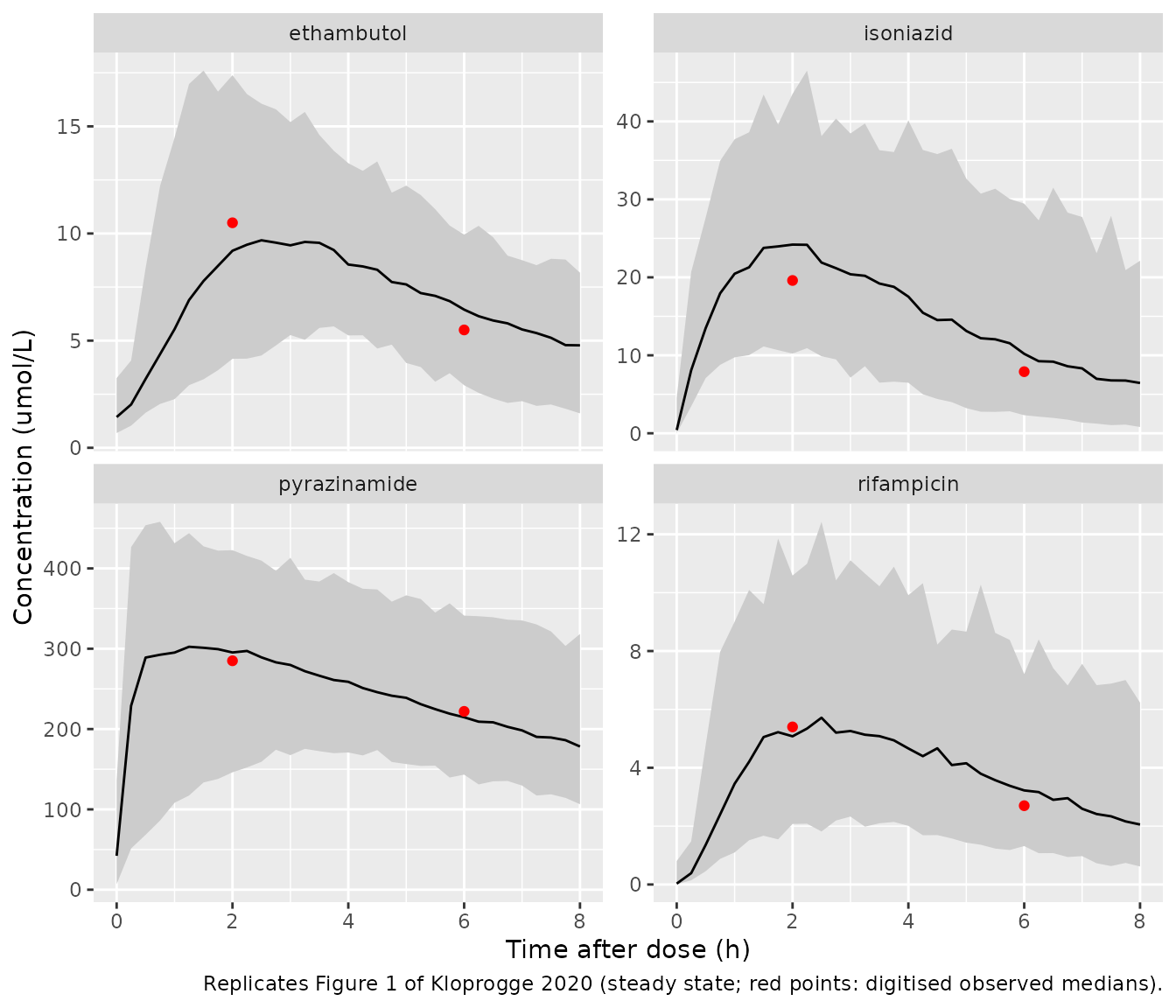
fig1_check <- pk_pct |>
  inner_join(fig1_obs, by = c("drug", "tad")) |>
  mutate(pct_diff = 100 * (p50 - median_umol) / median_umol)
fig1_check |>
  select(drug, tad, median_umol, p50, pct_diff) |>
  dplyr::rename(
    "Drug" = drug, "Time after dose (h)" = tad,
    "Observed median (umol/L)" = median_umol,
    "Simulated median (umol/L)" = p50, "% difference" = pct_diff
  ) |>
knitr::kable(digits = 1)| Drug | Time after dose (h) | Observed median (umol/L) | Simulated median (umol/L) | % difference |
|---|---|---|---|---|
| ethambutol | 2 | 10.5 | 9.2 | -12.4 |
| ethambutol | 6 | 5.5 | 6.4 | 17.2 |
| isoniazid | 2 | 19.6 | 24.2 | 23.5 |
| isoniazid | 6 | 7.9 | 10.2 | 29.0 |
| pyrazinamide | 2 | 285.0 | 295.3 | 3.6 |
| pyrazinamide | 6 | 222.0 | 214.7 | -3.3 |
| rifampicin | 2 | 5.4 | 5.1 | -6.0 |
| rifampicin | 6 | 2.7 | 3.2 | 19.4 |
# A wrong clearance, volume, dose or unit shifts the whole profile by tens of
# percent; the envelope is kept loose because the observed medians are
# digitised and pool day-14 and day-21 samples with off-nominal times.
stopifnot(
  abs(median(fig1_check$pct_diff)) < 20,
  all(abs(fig1_check$pct_diff) < 40)
)
NCA at steady state
conc_nca <- sim_pk |>
  filter(!is.na(Cc)) |>
  select(id, drug, tad, Cc)
dose_nca <- cohort |>
  tidyr::crossing(drugs |> select(drug, mg_per_tablet)) |>
  mutate(tad = 0, amt = tablets * mg_per_tablet) |>
  select(id, drug, tad, amt)

nca_res <- PKNCA::pk.nca(PKNCA::PKNCAdata(
  PKNCA::PKNCAconc(conc_nca, Cc ~ tad | drug + id),
  PKNCA::PKNCAdose(dose_nca, amt ~ tad | drug + id),
  intervals = data.frame(start = 0, end = 24, cmax = TRUE, auclast = TRUE)
))

# Model-derived medians for the study cohort (Results 'Pharmacokinetics';
# S1 Table): Cmax (mg/L) and AUC0-24 (h x mg/L).
published_nca <- data.frame(
  drug = c("isoniazid", "rifampicin", "pyrazinamide", "ethambutol"),
  cmax = c(3.24, 4.35, 40, 2.30),
  auclast = c(18.83, 29.10, 419, 18.50)
)

nca_tab <- nlmixr2lib::ncaComparisonTable(
  simulated = nca_res,
  reference = published_nca,
  by = "drug",
  params = c("cmax", "auclast"),
  units = c(cmax = "mg/L", auclast = "h*mg/L")
)
knitr::kable(nca_tab, caption = "AUClast is over the 0-24 h steady-state interval (AUC0-24).")| NCA parameter | drug | Reference | Simulated | % diff |
|---|---|---|---|---|
| Cmax (mg/L) | isoniazid | 3.24 | 3.43 | +5.9% |
| Cmax (mg/L) | rifampicin | 4.35 | 4.9 | +12.5% |
| Cmax (mg/L) | pyrazinamide | 40 | 40 | -0.1% |
| Cmax (mg/L) | ethambutol | 2.3 | 2.08 | -9.5% |
| AUClast (h*mg/L) | isoniazid | 18.8 | 21 | +11.5% |
| AUClast (h*mg/L) | rifampicin | 29.1 | 34.5 | +18.6% |
| AUClast (h*mg/L) | pyrazinamide | 419 | 422 | +0.8% |
| AUClast (h*mg/L) | ethambutol | 18.5 | 19.2 | +3.9% |
nca_med <- as.data.frame(nca_res$result) |>
  filter(PPTESTCD %in% c("cmax", "auclast")) |>
  group_by(drug, PPTESTCD) |>
  summarise(sim = median(PPORRES), .groups = "drop") |>
  inner_join(
    tidyr::pivot_longer(published_nca, -drug, names_to = "PPTESTCD", values_to = "ref"),
    by = c("drug", "PPTESTCD")
  ) |>
  mutate(pct_diff = 100 * (sim - ref) / ref)
stopifnot(
  abs(median(nca_med$pct_diff)) < 15,
  all(abs(nca_med$pct_diff) < 25)
)
The simulated cohort medians agree with the paper’s model-derived medians to within about 20%. The largest gap is rifampicin AUC0-24, which the simulation puts somewhat above the published 29.1 h x mg/L. The published values are medians of empirical Bayes estimates from sparse (three-sample) profiles, which shrink toward the typical value, so modest differences are expected.
Sputum bacillary-load PKPD model
Exposure covariates
The PKPD covariates are the individual steady-state AUC0-24 values. Here they come from the virtual PK cohort as dose / CL at steady state (the NCA AUClast over the dosing interval), converted to umol*h/L with the molecular weights 137.14 (isoniazid) and 822.94 (rifampicin) g/mol. To reach 200 patients, the 154-patient PK cohort is resampled with replacement. Baseline bilirubin is log-normal (median 7.5 umol/L, range 1-32) and 32% of patients report alcohol consumption, both as in Table 1.
auc_by_id <- as.data.frame(nca_res$result) |>
  filter(PPTESTCD == "auclast", drug %in% c("isoniazid", "rifampicin")) |>
  left_join(select(drugs, drug, mw), by = "drug") |>
  mutate(auc_umol = PPORRES / mw * 1000) |>
  select(id, drug, auc_umol) |>
  tidyr::pivot_wider(names_from = drug, values_from = auc_umol) |>
  rename(AUC_INH = isoniazid, AUC_RIF = rifampicin)

n_pd <- 200
pd_cohort <- tibble(
  id = seq_len(n_pd),
  pk_id = sample(auc_by_id$id, n_pd, replace = TRUE),
  TBILI = pmin(pmax(exp(rnorm(n_pd, log(7.5), 0.55)), 1), 32),
  ALCOHOL_USE = rbinom(n_pd, 1, 0.32)
) |>
  left_join(auc_by_id, by = c("pk_id" = "id")) |>
  select(-pk_id)

summary(select(pd_cohort, AUC_INH, AUC_RIF, TBILI))
#>     AUC_INH          AUC_RIF           TBILI
#>  Min.   : 46.81   Min.   : 16.00   Min.   : 1.466
#>  1st Qu.:114.54   1st Qu.: 34.47   1st Qu.: 5.176
#>  Median :145.79   Median : 41.65   Median : 7.701
#>  Mean   :165.48   Mean   : 43.31   Mean   : 9.105
#>  3rd Qu.:192.77   3rd Qu.: 48.83   3rd Qu.:11.090
#>  Max.   :604.30   Max.   :128.89   Max.   :32.000
The simulated isoniazid and rifampicin AUC ranges can be compared with the Figure 4 caption, which gives the study ranges as 54.9-515 and 19.9-145 h x umol/L.
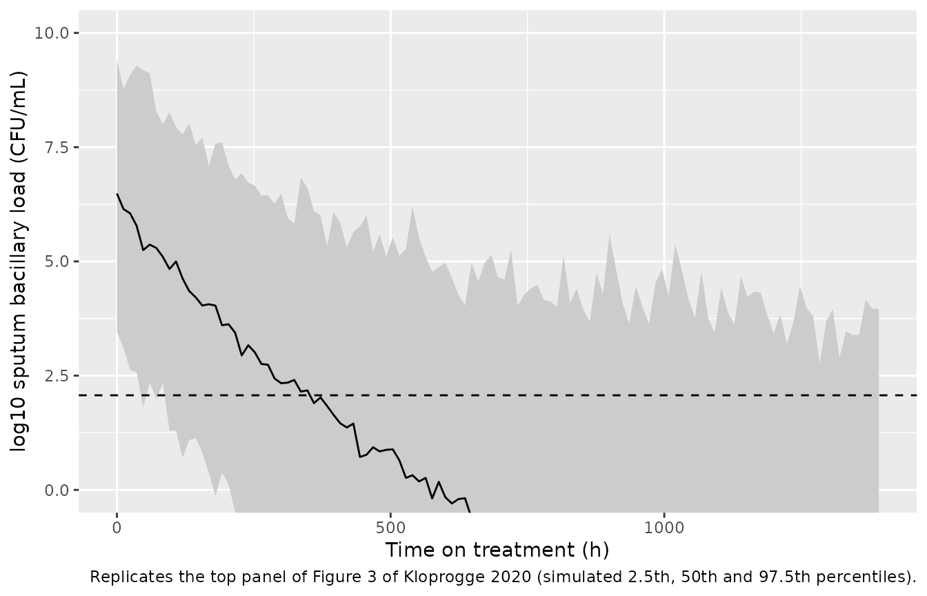
Replicating Figure 3 (VPC and fraction below the limit of quantification)
pd_mod <- readModelDb("Kloprogge_2020_hrze_bacterialload")
pd_times <- sort(unique(c(seq(0, 1400, by = 12), c(0, 2, 4, 7, 14, 28, 49, 56) * 24)))
pd_events <- pd_cohort |>
  tidyr::crossing(time = pd_times) |>
  mutate(evid = 0L, amt = NA_real_, cmt = "cfu") |>
  arrange(id, time)

sim_pd <- rxode2::rxSolve(pd_mod, events = pd_events) |>
  as.data.frame()
#> ℹ parameter labels from comments will be replaced by 'label()'

lloq <- 2.07 # log10 CFU/mL; the LLOQ reference line of Figure 3, digitised
pd_pct <- sim_pd |>
  group_by(time) |>
  summarise(
    p025 = quantile(sim, 0.025),
    p50 = median(sim),
    p975 = quantile(sim, 0.975),
    # Expected fraction of samples below the LLOQ: the residual error is
    # integrated analytically around each individual prediction.
    p_blq = mean(pnorm((lloq - log_cfu) / 1.607)),
    .groups = "drop"
  )

ggplot(pd_pct, aes(time)) +
  geom_ribbon(aes(ymin = p025, ymax = p975), fill = "grey80") +
  geom_line(aes(y = p50)) +
  geom_hline(yintercept = lloq, linetype = "dashed") +
  coord_cartesian(ylim = c(0, 10)) +
  labs(
    x = "Time on treatment (h)", y = "log10 sputum bacillary load (CFU/mL)",
    caption = "Replicates the top panel of Figure 3 of Kloprogge 2020 (simulated 2.5th, 50th and 97.5th percentiles)."
  )
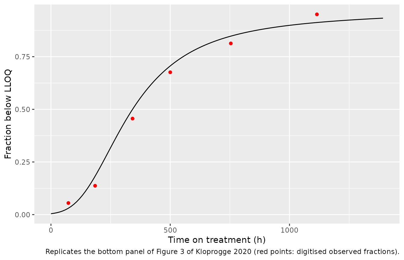
The lower panel of Figure 3 gives the observed fraction of samples below the limit of quantification in each time bin. The maintainers digitised those fractions and compare them with the model-expected fraction at the bin centres.
fig3_blq <- tibble(
  time = c(73, 185, 342, 500, 754, 1115),
  observed = c(0.055, 0.137, 0.456, 0.676, 0.813, 0.951)
)
blq_check <- fig3_blq |>
  mutate(
    simulated = approx(pd_pct$time, pd_pct$p_blq, xout = time)$y,
    difference = simulated - observed
  )

ggplot(pd_pct, aes(time, p_blq)) +
  geom_line() +
  geom_point(data = fig3_blq, aes(y = observed), colour = "red") +
  labs(
    x = "Time on treatment (h)", y = "Fraction below LLOQ",
    caption = "Replicates the bottom panel of Figure 3 of Kloprogge 2020 (red points: digitised observed fractions)."
  )
blq_check |>
  dplyr::rename(
    "Time (h)" = time, "Observed fraction" = observed,
    "Simulated fraction" = simulated, "Difference" = difference
  ) |>
knitr::kable(digits = 3)| Time (h) | Observed fraction | Simulated fraction | Difference |
|---|---|---|---|
| 73 | 0.055 | 0.030 | -0.025 |
| 185 | 0.137 | 0.182 | 0.045 |
| 342 | 0.456 | 0.500 | 0.044 |
| 500 | 0.676 | 0.706 | 0.030 |
| 754 | 0.813 | 0.848 | 0.035 |
| 1115 | 0.951 | 0.912 | -0.039 |
# Robust to cohort draw: the per-bin fractions of a 200-patient cohort vary
# by a few percentage points; a mis-specified BETA distribution (log-normal,
# see Assumptions) caps the late fraction near 0.6 and fails this at once.
stopifnot(
  abs(median(blq_check$difference)) < 0.08,
  quantile(abs(blq_check$difference), 0.9) < 0.15
)
Replicating Figure 4 (covariate effects on the typical profile)
Figure 4 shows population-predicted CFU with one covariate at its study extreme and the others at their medians, with and without alcohol consumption. The maintainers digitised the end point of each curve.
fig4_scen <- tribble(
  ~panel, ~exposure, ~AUC_INH, ~AUC_RIF, ~TBILI,
  "Baseline bilirubin", "High", 137.3, 35.36, 32,
  "Baseline bilirubin", "Low", 137.3, 35.36, 1,
  "Isoniazid", "High", 515, 35.36, 7.5,
  "Isoniazid", "Low", 54.9, 35.36, 7.5,
  "Rifampicin", "High", 137.3, 145, 7.5,
  "Rifampicin", "Low", 137.3, 19.9, 7.5
) |>
  tidyr::crossing(ALCOHOL_USE = c(0, 1)) |>
  mutate(id = row_number())

fig4_events <- fig4_scen |>
  tidyr::crossing(time = seq(0, 1020, by = 4)) |>
  mutate(evid = 0L, amt = NA_real_, cmt = "cfu") |>
  arrange(id, time)
sim_fig4 <- rxode2::rxSolve(rxode2::zeroRe(pd_mod), events = fig4_events) |>
  as.data.frame() |>
  select(id, time, log_cfu) |>
  left_join(select(fig4_scen, id, panel, exposure, ALCOHOL_USE), by = "id") |>
  mutate(alcohol = ifelse(ALCOHOL_USE == 1, "Alcohol", "No alcohol"))
#> ℹ parameter labels from comments will be replaced by 'label()'
#> ℹ omega/sigma items treated as zero: 'etalt12', 'etalogitbeta', 'etallam', 'etae0_cfu'
#> Warning: multi-subject simulation without without 'omega'

ggplot(sim_fig4, aes(time, 10^log_cfu, colour = exposure, linetype = alcohol)) +
  geom_line() +
  scale_y_log10() +
  facet_wrap(~panel) +
  labs(
    x = "Time (h)", y = "Population predicted CFU/mL", colour = NULL, linetype = NULL,
    caption = "Replicates Figure 4 of Kloprogge 2020."
  )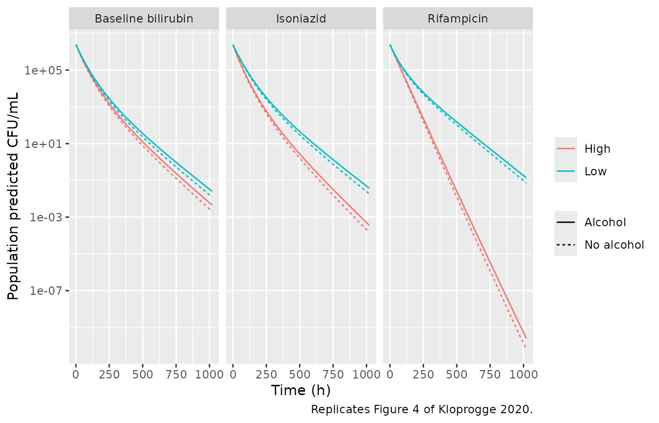
fig4_digitised <- tribble(
  ~panel, ~exposure, ~ALCOHOL_USE, ~time, ~log_cfu_fig,
  "Baseline bilirubin", "High", 1, 672, -0.09,
  "Baseline bilirubin", "High", 0, 672, -0.34,
  "Baseline bilirubin", "Low", 1, 840, -0.55,
  "Baseline bilirubin", "Low", 0, 840, -0.79,
  "Isoniazid", "High", 1, 672, -0.90,
  "Isoniazid", "High", 0, 500, 0.21,
  "Isoniazid", "Low", 1, 844, -0.40,
  "Isoniazid", "Low", 0, 844, -0.69,
  "Rifampicin", "High", 1, 336, 1.00,
  "Rifampicin", "High", 0, 336, 0.82,
  "Rifampicin", "Low", 1, 1008, -0.79,
  "Rifampicin", "Low", 0, 844, -0.06
)
interp_curve <- function(curve_id, at_time) {
  d <- sim_fig4[sim_fig4$id == curve_id, ]
  approx(d$time, d$log_cfu, xout = at_time)$y
}
fig4_check <- fig4_digitised |>
  left_join(fig4_scen |> select(id, panel, exposure, ALCOHOL_USE), by = c("panel", "exposure", "ALCOHOL_USE")) |>
  mutate(
    log_cfu_model = mapply(interp_curve, id, time),
    difference = log_cfu_model - log_cfu_fig
  )

fig4_check |>
  select(panel, exposure, ALCOHOL_USE, time, log_cfu_fig, log_cfu_model, difference) |>
  dplyr::rename(
    "Panel" = panel, "Exposure" = exposure, "Alcohol" = ALCOHOL_USE, "Time (h)" = time,
    "Figure 4 (log10 CFU/mL)" = log_cfu_fig, "Model (log10 CFU/mL)" = log_cfu_model,
    "Difference" = difference
  ) |>
knitr::kable(digits = 2)| Panel | Exposure | Alcohol | Time (h) | Figure 4 (log10 CFU/mL) | Model (log10 CFU/mL) | Difference |
|---|---|---|---|---|---|---|
| Baseline bilirubin | High | 1 | 672 | -0.09 | -0.10 | -0.01 |
| Baseline bilirubin | High | 0 | 672 | -0.34 | -0.36 | -0.02 |
| Baseline bilirubin | Low | 1 | 840 | -0.55 | -0.55 | 0.00 |
| Baseline bilirubin | Low | 0 | 840 | -0.79 | -0.82 | -0.03 |
| Isoniazid | High | 1 | 672 | -0.90 | -0.91 | -0.01 |
| Isoniazid | High | 0 | 500 | 0.21 | 0.20 | -0.01 |
| Isoniazid | Low | 1 | 844 | -0.40 | -0.42 | -0.02 |
| Isoniazid | Low | 0 | 844 | -0.69 | -0.69 | 0.00 |
| Rifampicin | High | 1 | 336 | 1.00 | 0.99 | -0.01 |
| Rifampicin | High | 0 | 336 | 0.82 | 0.78 | -0.04 |
| Rifampicin | Low | 1 | 1008 | -0.79 | -0.79 | 0.00 |
| Rifampicin | Low | 0 | 844 | -0.06 | -0.08 | -0.02 |
Assumptions and deviations
- Allometric exponents. The supplement states that body weight enters clearance and volume “using allometry” around a drug-specific reference weight, without printing the exponents. The standard 0.75 (clearances) and 1 (volumes) are used. They are the exponents of each drug’s source model (Seng 2015, Sloan 2017, Alsultan 2017, Jonsson 2011), whose reference weights Kloprogge 2020 adopted. For the two-compartment drugs, scaling is applied to Q/F and Vp/F as well as CL/F and Vc/F, as in the source models.
- Rifampicin sex effect. ‘Cl~Male’ = 0.183 is applied as a log-scale effect of male sex, so females are the reference. The supplement says that rifampicin clearance was “centralised around male patients”. The maintainers read this as describing the male-sex covariate, for three reasons: the parameter is named for males; exp(0.183) = 1.20 matches the male/female ratio of Sloan 2017 in the same cohort; and the female-reference reading gives a cohort median AUC0-24 closer to the published 29.1 h x mg/L.
- Ethambutol transit count. S1 Table gives MTT but no transit count for ethambutol. The single transit compartment ahead of the absorption compartment (ktr = 1/MTT) of Jonsson 2011 is used, because MTT and ka were fixed to that model.
- Pyrazinamide additive error. S1 Table prints 74.5 with no unit. The Figure 1 VPC shows that the data were in umol/L. Read as an SD of 74.5 umol/L, it puts the simulated 2.5th percentile of predose concentrations well below zero and the 6-h 2.5th percentile near half the observed value. It is therefore read as a NONMEM variance: SD = sqrt(74.5) = 8.63 umol/L = 1.063 mg/L (close to the 0.94 mg/L of Alsultan 2017).
- Concentration units. The analysis dataset was in umol/L (Figure 1). The packaged PK models take doses in mg and return mg/L; clearances and volumes do not depend on the unit.
- PKPD residual error. S2 Table ‘RUV’ = 2.5832 is taken as the NONMEM variance (SD 1.607 log10 CFU/mL). This reproduces the Figure 3 baseline spread, which an SD of 2.58 would not.
- BETA distribution. The supplement states that all PKPD parameters except the baseline were log-normal. But S2 Table bounds BETA to [0, 1], and a log-normal BETA with variance 1.31 exceeds 1 in about 35% of patients, which would make those patients’ bacterial load regrow. Under that reading the simulated fraction below the LLOQ plateaus near 0.6 and the 97.5th percentile rises past 50 log10 CFU/mL. Figure 3 shows 95% of samples below the LLOQ by 1100 h and an upper band near 5 log10 CFU/mL. The BETA IIV is therefore placed on the logit scale, which reproduces Figure 3.
- Sign of knet. The printed knet equation carries a leading minus sign that, combined with dB/dt = -knet B, would make the load grow. The decline described throughout the paper is used.
- Covariate centring. The continuous PKPD covariates are centred on their medians. The PKPD-cohort median bilirubin (7.5 umol/L) is in Table 1, but the PKPD-cohort AUC medians are not printed. The PK-cohort medians of 18.83 and 29.10 h x mg/L are used, converted to 137.3 and 35.36 h x umol/L. The Figure 4 end points are reproduced within digitisation accuracy with these values.
- Units of the AUC covariates. The Figure 4 caption gives the covariate ranges in h x umol/L, which matches the PK-cohort mg-based ranges once they are converted with the molecular weights.
- Below-LLOQ handling. The paper fitted the counts below the limit of quantification with the M3 method. The packaged model has a plain additive residual on log10 CFU/mL; the vignette computes the expected fraction below the LLOQ (2.07 log10 CFU/mL, digitised from Figure 3) analytically.
- Exposure-response scope. The authors caution that the concentration range was restricted by standard dosing, so the PKPD model is descriptive and not suitable for dose extrapolation (Discussion). The outcome analyses (univariate logistic and Cox regressions of failure and recurrence, Tables 2 and 3) are statistical screens without a reported model for simulation and are not packaged.