Fospropofol (Gibiansky 2005)
Source:vignettes/articles/Gibiansky_2005_fospropofol.Rmd
Gibiansky_2005_fospropofol.RmdModel and source
- Citation: Gibiansky E, Gibiansky L, Enriquez J. Population pharmacokinetic model of sedative doses of GPI 15715 and propofol liberated from GPI 15715. Clin Pharmacol Ther. 2005;77(2):P32 (PII-87, ASCPT Annual Meeting poster). doi:10.1016/j.clpt.2004.12.076. Poster PDF hosted at https://metrumrg.com/wp-content/uploads/2018/08/ascpt_2005_ppkmodelgpi.pdf
- Description: Joint two-compartment fospropofol (GPI 15715, AQUAVAN) prodrug + intermediate delay compartment + two-compartment propofol active-metabolite population PK model in adults receiving IV bolus AQUAVAN for procedural sedation (Gibiansky 2005, ASCPT poster, colonoscopy sedation Phase II study). The model assumes complete metabolism of GPI 15715 to propofol via systemic alkaline-phosphatase hydrolysis; the intermediate compartment captures the appearance delay between GPI 15715 elimination from plasma and the corresponding rise in propofol concentration. Lean body mass (LBM, reference 55 kg) was retained as a linear-fractional covariate on GPI 15715 central volume Vc_GPI, GPI 15715 metabolic clearance CL_GPI, and propofol central volume Vc_PR; fentanyl premedication exposure, age, sex, and other demographics/laboratory covariates were tested but not retained. Propofol Vc_PR (6.91 L) was fixed as the data were insufficient for joint estimation with CL_PR (the model is identifiable on CL_PR = K10_PR * Vc_PR = 4.53 L/min).
- Poster: https://metrumrg.com/wp-content/uploads/2018/08/ascpt_2005_ppkmodelgpi.pdf
- Abstract DOI: https://doi.org/10.1016/j.clpt.2004.12.076
The packaged model implements the Gibiansky 2005 joint two-compartment prodrug (GPI 15715, fospropofol, AQUAVAN) + intermediate delay compartment + two-compartment active-metabolite (propofol) population PK model, fitted in 158 adults receiving IV bolus AQUAVAN for procedural sedation during elective colonoscopy. The source is an ASCPT 2005 Annual Meeting poster authored by Gibiansky, Gibiansky, and Enriquez of Guilford Pharmaceuticals and Metrum Research Group; no peer-reviewed journal article expands on the model. Complete metabolism of GPI 15715 to propofol via systemic alkaline-phosphatase hydrolysis is assumed; the intermediate delay compartment captures the appearance lag between GPI 15715 elimination from plasma and the corresponding rise in propofol concentration. Lean body mass (LBM, reference 55 kg) is the only retained covariate (linear-fractional on Vc_GPI, CL_GPI, and Vc_PR); the propofol central volume Vc_PR was fixed at 6.91 L because the data were insufficient for joint estimation with CL_PR (the model is identifiable on CL_PR = K10_PR * Vc_PR = 4.53 L/min). The model parameters are parameterised with rate constants (K12_GPI, K21_GPI, K_GPI-PR, K10_PR, K12_PR, K21_PR) rather than canonical CL / Q / Vp so the poster’s IIV variance / covariance block (Table 2) can be carried verbatim without cross-parameter covariance translation.
Population
The model was fitted to 597 GPI 15715 and 599 propofol plasma concentrations from 158 adults (69 male, 89 female; age 20-85 years, 18 patients > 65 y; total body weight 45-140 kg; lean body weight 37-81 kg) enrolled in a single randomised, open-label, Phase II dose-ranging colonoscopy sedation study. Each patient received an intravenous fentanyl citrate premedication dose (0.5 to 1.5 ug/kg, cumulative 11-201 ug) 5 minutes before an AQUAVAN IV bolus (7.5 to 12.5 mg/kg) followed by up to four supplemental AQUAVAN doses (each approximately 25% of the initial bolus, occasionally 50%, with at least 3 minutes between doses) for inducing and maintaining sedation through the procedure. The total cumulative AQUAVAN dose ranged from 495 to 1,680 mg across the cohort. Four venous blood samples per patient were drawn for GPI 15715 and propofol plasma determinations.
Covariate testing included demographics (gender, total body weight,
age, race, body surface area, lean body weight, body mass index),
laboratory values (albumin, alanine transaminase, aspartate
transaminase, total bilirubin, estimated creatinine clearance, alkaline
phosphatase), fentanyl exposure (initial and total doses,
weight-normalised doses, plasma concentrations at 1 and 9 minutes), and
AQUAVAN dose (total and weight-normalised). Only LBM was retained in the
final model. Gender was strongly co-linear with WT and LBM, and was not
retained as an independent effect after adjustment for LBM. Fentanyl
exposure did not affect either GPI 15715 or propofol PK. Older age (>
65 y) was not associated with PK changes, although the > 65 y stratum
comprises only 18 patients (about 11% of the cohort), so the absence of
an age effect is moderately powered. The same metadata is available
programmatically via
readModelDb("Gibiansky_2005_fospropofol")$meta$population.
Source trace
The per-parameter origin is recorded as an in-file comment next to
each ini() entry in
inst/modeldb/specificDrugs/Gibiansky_2005_fospropofol.R.
The table below collects them in one place for review. All point
estimates are from Gibiansky 2005 poster Table 1 (Fixed-Effect
Parameters of the Final PK Model); all IIV omega and covariance
estimates and residual error variance estimates are from poster Table 2
(Random-Effect Parameters). The structural-model layout is from poster
Figure 2; the LBM-covariate parameterisation is from the Results /
Covariate Effects section; the residual-error model form
(Ln(Y) = Ln(F) + W * eps with
W^2 = theta1 / F^2 + theta2) is from the Methods / Error
Models section.
| Equation / parameter | Value | Source location |
|---|---|---|
lvc (Vc_GPI) |
log(6.08) -> 6.08 L (LBM 55 kg) | Table 1: Vc_GPI = 6.08, RSE 4.6% |
lcl (CL_GPI metabolic) |
log(0.298) -> 0.298 L/min (LBM 55) | Table 1: CL_GPI = 0.298, RSE 8.0% |
lk12 (K12_GPI) |
log(0.0198) -> 0.0198 1/min | Table 1: K12_GPI = 0.0198, RSE 24% |
lk21 (K21_GPI) |
log(0.00617) -> 0.00617 1/min | Table 1: K21_GPI = 0.00617, RSE 21% |
lka_ppf (K_GPI-PR) |
log(0.982) -> 0.982 1/min | Table 1: K_GPI-PR = 0.982, RSE 14% |
lvc_ppf (Vc_PR, fixed) |
fixed(log(6.91)) -> 6.91 L | Table 1 footnote: Vc_PR FIXED |
lk10_ppf (K10_PR) |
log(0.655) -> 0.655 1/min | Table 1: K10_PR = 0.655, RSE 8.0% |
lk12_ppf (K12_PR) |
log(0.732) -> 0.732 1/min | Table 1: K12_PR = 0.732, RSE 11% |
lk21_ppf (K21_PR) |
log(0.0383) -> 0.0383 1/min | Table 1: K21_PR = 0.0383, RSE 20% |
e_lbm_vc (LBM on Vc_GPI) |
0.0194 per kg from 55 | Table 1 / Results: 1.8%/kg (Table 1 prints 0.194, see Errata below) |
e_lbm_cl (LBM on CL_GPI) |
0.0270 per kg from 55 | Table 1 / Results: 2.5%/kg (Table 1 prints 0.270, see Errata below) |
e_lbm_vc_ppf (LBM on Vc_PR) |
0.0155 per kg from 55 | Table 1 / Results: 1.4%/kg (Table 1 prints 0.155, see Errata below) |
etalvc variance |
0.0727 (CV 27.5%) | Table 2: omega^2(Vc_GPI), RSE 29% |
etalka_ppf variance |
1.0 (CV 131%, near boundary) | Table 2: omega^2(K_GPI-PR), RSE 23% |
etalk12 variance |
1.04 (CV 135%, near boundary) | Table 2: omega^2(K12_GPI), RSE 49% |
etalvc_ppf variance |
0.0699 (CV 26.9%) | Table 2: omega^2(Vc_PR), RSE 29% |
cov(etalvc, etalka_ppf) |
-0.239 (R = -0.886) | Table 2: omega(Vc_GPI, K_GPI-PR), RSE 15% |
cov(etalka_ppf, etalk12) |
0.271 (R = 0.266) | Table 2: omega(K_GPI-PR, K12_GPI), RSE 46% |
cov(etalk12, etalvc_ppf) |
-0.136 (R = -0.504) | Table 2: omega(K12_GPI, Vc_PR), RSE 48% |
addSd (GPI add residual) |
2.74 ug/mL | Table 2: sigma^2_GPI_ADD = 7.52, SD = 2.74, RSE 44% |
propSd (GPI prop residual) |
0.40 (CV 40.0%) | Table 2: sigma^2_GPI_PROP = 0.16, RSE 20% |
addSd_ppf (PR add residual) |
0.104 ug/mL | Table 2: sigma^2_PR_ADD = 0.0109, SD = 0.104, RSE 33% |
propSd_ppf (PR prop) |
0.378 (CV 37.8%) | Table 2: sigma^2_PR_PROP = 0.143, RSE 12% |
ODE: d/dt(central)
|
-kel*central - k12*central + k21*peripheral1 |
Figure 2 + Results |
ODE: d/dt(peripheral1)
|
k12*central - k21*peripheral1 |
Figure 2 + Results |
ODE: d/dt(delay)
|
kel*central - ka_ppf*delay |
Figure 2 + Results (intermediate compartment) |
ODE: d/dt(central_ppf)
|
ka_ppf*delay - k10_ppf*central_ppf - k12_ppf*central_ppf + k21_ppf*peripheral1_ppf |
Figure 2 + Results |
ODE: d/dt(peripheral1_ppf)
|
k12_ppf*central_ppf - k21_ppf*peripheral1_ppf |
Figure 2 + Results |
Virtual cohort
Original observed plasma concentrations are not publicly available. The figures below use a virtual population whose LBM distribution matches the LBM strata called out by Figure 3 of the poster (35, 55, and 85 kg) at the fixed 800 mg AQUAVAN bolus the poster uses for the Figure 3 demonstration. Each LBM stratum carries 100 simulated subjects (well below the per-arm cap of 200), and the random-effects draws use the published IIV variance / covariance block (Table 2) so the cohort spread reflects the published population variability.
set.seed(20050101)

mod <- rxode2::rxode(readModelDb("Gibiansky_2005_fospropofol"))

n_per_arm  <- 100L
dose_mg    <- 800   # AQUAVAN bolus matching poster Figure 3
obs_times  <- c(0.25, 0.5, 0.75, 1, 1.5, 2, 2.5, 3, 4, 5, 6, 7, 8, 9, 10,
                12, 15, 20, 25, 30, 40, 50, 60, 75, 90, 105, 120)

# Helper: one cohort = one LBM stratum. Subjects in the same cohort
# share LBM and the 800 mg bolus; id_offset keeps subject IDs disjoint
# across cohorts so bind_rows() doesn't collapse them. The model has
# two observation outputs (Cc for GPI 15715 and Cc_ppf for propofol)
# so each observation time carries two rows: dvid = 1 (Cc) and
# dvid = 2 (Cc_ppf). The dvid->observable mapping is the order of the
# residual-error declarations in the model() block; rxSolve auto-
# generates the mapping from the rxUi.
make_cohort <- function(n, lbm, lbm_label, id_offset = 0L) {
  ids  <- id_offset + seq_len(n)
  base <- tibble(id = ids, LBM = lbm, lbm_label = lbm_label)
  doses <- base |>
    mutate(time = 0, amt = dose_mg, evid = 1L,
           cmt = "central", dvid = NA_integer_)
  obs <- tidyr::crossing(id = ids, time = obs_times,
                         dvid = c(1L, 2L)) |>
    mutate(evid = 0L, amt = NA_real_, cmt = NA_character_) |>
    left_join(base, by = "id")
  bind_rows(doses, obs) |>
    arrange(id, time, desc(evid), dvid)
}

events <- bind_rows(
  make_cohort(n_per_arm, lbm = 35, lbm_label = "LBM 35 kg",
              id_offset = 0L * n_per_arm),
  make_cohort(n_per_arm, lbm = 55, lbm_label = "LBM 55 kg (reference)",
              id_offset = 1L * n_per_arm),
  make_cohort(n_per_arm, lbm = 85, lbm_label = "LBM 85 kg",
              id_offset = 2L * n_per_arm)
)
stopifnot(!anyDuplicated(unique(events[, c("id", "time", "evid", "dvid")])))
Simulation
Two simulation runs are produced. The typical-value run sets all random effects to zero so the LBM-driven shifts are isolated; this is the simulation that replicates the poster Figure 3 right-panel “Cmax_PR vs LBW” panel exactly because Figure 3 itself is a typical-value comparison at a fixed 800 mg dose. The stochastic run draws random effects from the published IIV variance / covariance block (Table 2) and is used for the VPC overlay and for the PKNCA validation table further below.
sim_typical <- rxode2::rxSolve(
  object  = rxode2::zeroRe(mod),
  events  = events,
  keep    = c("LBM", "lbm_label"),
  returnType = "data.frame"
)
#> ℹ omega/sigma items treated as zero: 'etalvc_ppf', 'etalk12', 'etalka_ppf', 'etalvc'
#> Warning: multi-subject simulation without without 'omega'

sim_stochastic <- rxode2::rxSolve(
  object  = mod,
  events  = events,
  keep    = c("LBM", "lbm_label"),
  returnType = "data.frame"
)
Replicate published figures
Gibiansky 2005 Figure 3 – propofol concentration and Cmax vs LBM (800 mg bolus)
Figure 3 of the poster shows two panels at a fixed 800 mg AQUAVAN bolus: the left panel plots propofol concentration vs time for LBW strata 35, 45, 55, 65, 75, and 85 kg (an overlay of six smooth typical-value curves), and the right panel plots propofol Cmax against LBW across the same strata. The poster narrative states that Cmax is “20% higher in patients with LBW of 35 kg” and “20% lower in patients with LBW of 85 kg” relative to the 55 kg reference patient. The replication below carries the three reference strata used by the poster narrative (35, 55, 85 kg) and reads off both the concentration-time profile and the LBM-vs-Cmax relationship.
sim_typical |>
  mutate(lbm_label = factor(lbm_label,
                            levels = c("LBM 35 kg",
                                       "LBM 55 kg (reference)",
                                       "LBM 85 kg"))) |>
  filter(time > 0) |>
  ggplot(aes(time, Cc_ppf, colour = lbm_label)) +
    geom_line(linewidth = 0.9) +
    labs(x = "Time post AQUAVAN bolus (min)",
         y = "Propofol Cc (ug/mL)",
         colour = NULL,
         title = "Figure 3 left panel -- propofol concentration over time vs LBM",
         caption = "800 mg AQUAVAN bolus; typical-value simulation (zero random effects). Replicates Gibiansky 2005 Figure 3 left panel for the three reference strata.")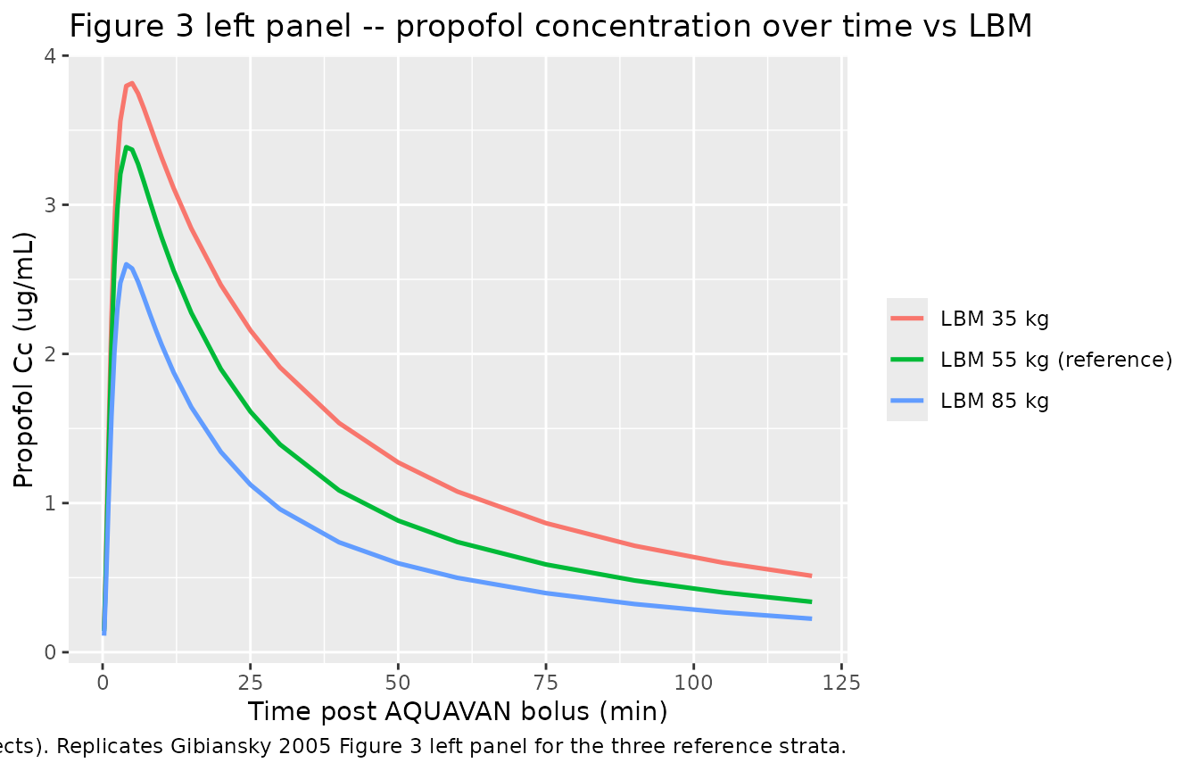
cmax_by_lbm <- sim_typical |>
  filter(time > 0) |>
  group_by(LBM, lbm_label) |>
  summarise(cmax_ppf = max(Cc_ppf, na.rm = TRUE), .groups = "drop")

cmax_ref <- cmax_by_lbm |>
  filter(LBM == 55) |>
  pull(cmax_ppf)

cmax_by_lbm <- cmax_by_lbm |>
  mutate(pct_vs_ref = 100 * (cmax_ppf - cmax_ref) / cmax_ref)

ggplot(cmax_by_lbm, aes(LBM, cmax_ppf)) +
  geom_point(size = 3, colour = "steelblue") +
  geom_text(aes(label = sprintf("%+.1f%%", pct_vs_ref)),
            vjust = -1.0, size = 3.5) +
  scale_x_continuous(breaks = c(35, 55, 85)) +
  expand_limits(y = max(cmax_by_lbm$cmax_ppf) * 1.10) +
  labs(x = "Lean body mass (kg)",
       y = "Propofol Cmax (ug/mL)",
       title = "Figure 3 right panel -- propofol Cmax vs LBM (800 mg bolus)",
       caption = "Typical-value simulation. Labels show percent change vs the LBM = 55 kg reference. Replicates Gibiansky 2005 Figure 3 right panel.")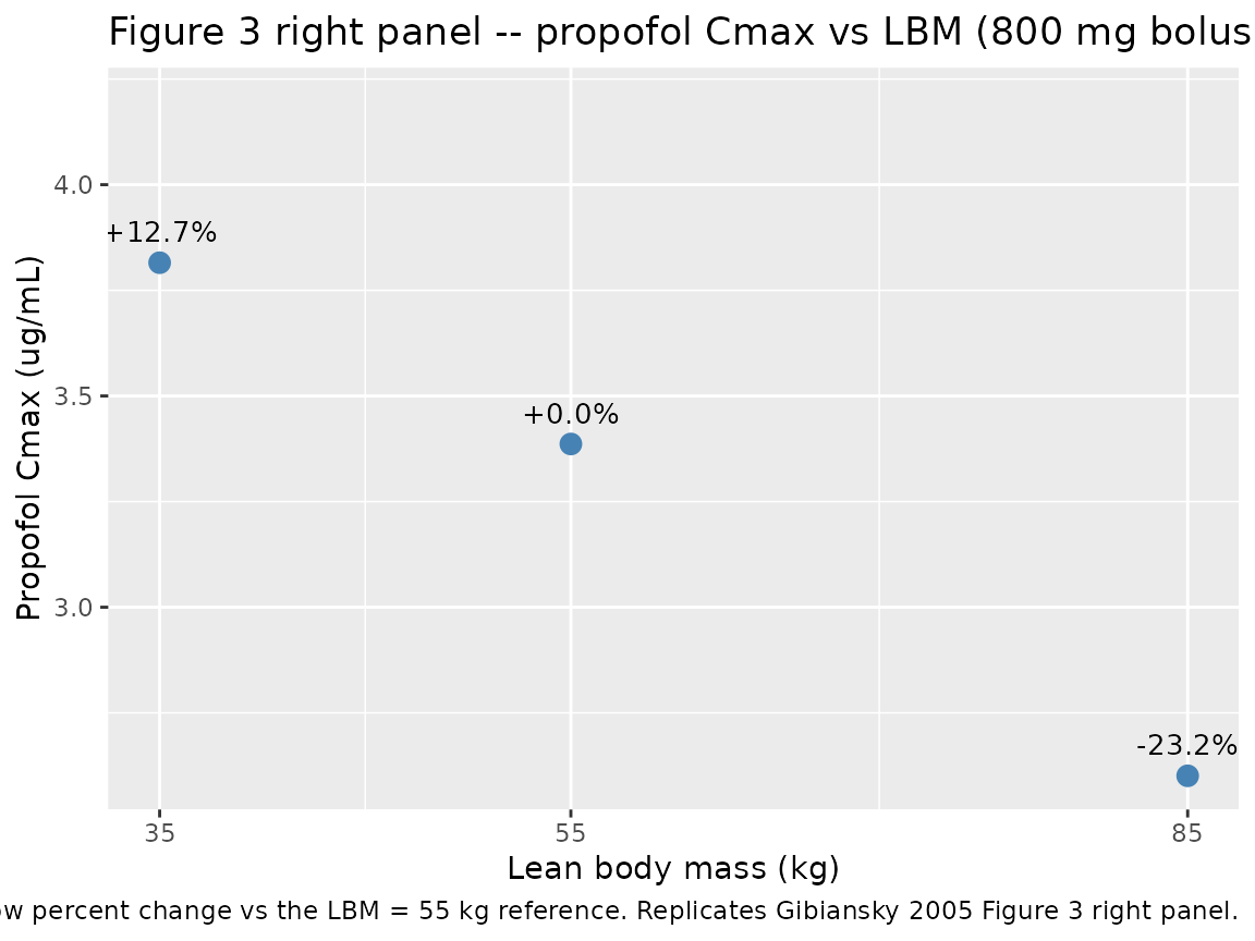
The poster narrative quotes “Cmax 20% higher at LBW 35 kg” and “Cmax 20% lower at LBW 85 kg” relative to the 55 kg reference. The percent-change labels printed on the figure above show the simulated values for direct comparison.
VPC – stochastic concentration ribbons at LBM 55 kg
The 90% prediction band of the 100-subject stochastic simulation at LBM = 55 kg overlays the typical-value curve for both analytes. The band reflects the published IIV variance / covariance block (Table 2) of the poster, which is dominated by the boundary-hitting variances on K_GPI-PR and K12_GPI (CV 131-135%); the propofol concentration ribbon is therefore relatively wide.
ribbon_df <- sim_stochastic |>
  filter(lbm_label == "LBM 55 kg (reference)", time > 0) |>
  pivot_longer(c(Cc, Cc_ppf), names_to = "analyte", values_to = "conc") |>
  group_by(analyte, time) |>
  summarise(
    Q05 = quantile(conc, 0.05, na.rm = TRUE),
    Q50 = quantile(conc, 0.50, na.rm = TRUE),
    Q95 = quantile(conc, 0.95, na.rm = TRUE),
    .groups = "drop"
  ) |>
  mutate(analyte = factor(analyte,
                          levels = c("Cc", "Cc_ppf"),
                          labels = c("GPI 15715", "Propofol")))

typ_df <- sim_typical |>
  filter(lbm_label == "LBM 55 kg (reference)", time > 0) |>
  pivot_longer(c(Cc, Cc_ppf), names_to = "analyte", values_to = "conc") |>
  mutate(analyte = factor(analyte,
                          levels = c("Cc", "Cc_ppf"),
                          labels = c("GPI 15715", "Propofol")))

ggplot(ribbon_df, aes(time, Q50)) +
  geom_ribbon(aes(ymin = Q05, ymax = Q95), alpha = 0.25, fill = "steelblue") +
  geom_line(linewidth = 0.7, colour = "steelblue") +
  geom_line(data = typ_df, aes(time, conc),
            linetype = 2, linewidth = 0.6, colour = "black") +
  facet_wrap(~ analyte, scales = "free_y") +
  labs(x = "Time post AQUAVAN bolus (min)",
       y = "Plasma concentration (ug/mL)",
       title = "Stochastic VPC at LBM = 55 kg, 800 mg AQUAVAN bolus",
       caption = "Solid steelblue = stochastic median; ribbon = 5th-95th percentile (100 simulated subjects); dashed black = typical-value (zero random effects).")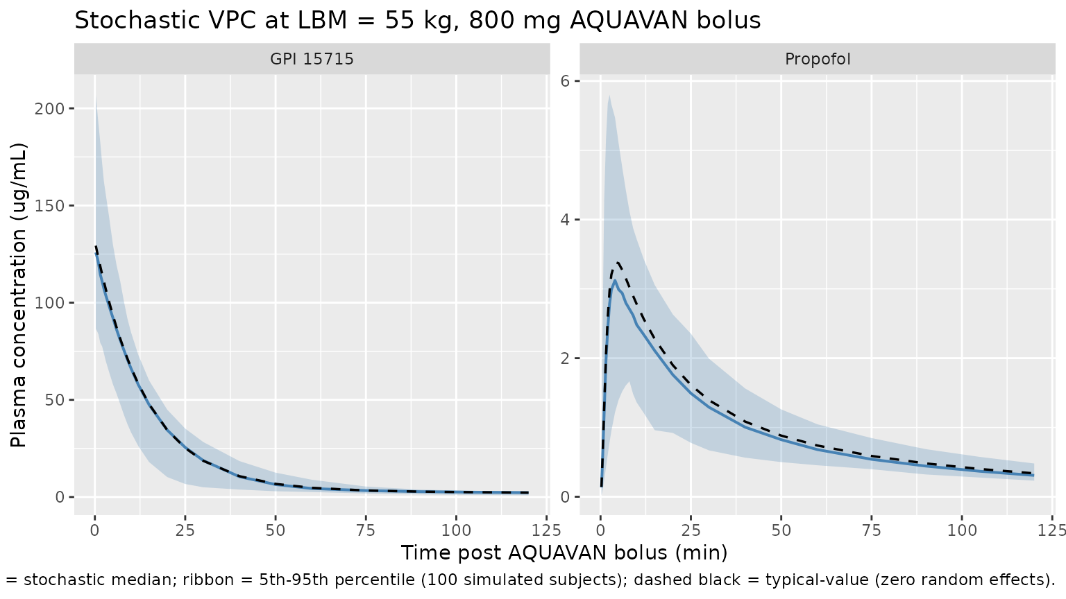
PKNCA validation
PKNCA computes Cmax, Tmax, and AUC-to-infinity over a single-bolus
single-dose interval, separately for the GPI 15715 (Cc) and
propofol (Cc_ppf) outputs. Each block keeps the LBM stratum
(lbm_label) in the PKNCAconc formula so the per-stratum NCA
summary can be inspected. The stochastic-simulation cohort is used so
the NCA spread reflects the published IIV variance / covariance block;
the typical-value Cmax is reported separately in the Figure 3 right
panel above.
# PKNCA helper: one analyte, one event/sim pair, treatment-stratified
# by lbm_label. The simulation grid already includes time = 0 (the dose
# row carries it), but rxSolve sometimes emits the post-dose grid only;
# the defensive `bind_rows` ensures every (id, treatment) has a t = 0
# row at 0 ug/mL (true for an IV bolus before the dose lands) so PKNCA
# does not warn about the AUC window starting before the first
# measurement.
nca_one_analyte <- function(sim, events, conc_col, conc_label) {
  conc_df <- sim |>
    dplyr::filter(!is.na(.data[[conc_col]])) |>
    dplyr::select(id, time, lbm_label, dplyr::all_of(conc_col))
  colnames(conc_df)[colnames(conc_df) == conc_col] <- "Cc"
  conc_df <- dplyr::bind_rows(
    conc_df,
    conc_df |> dplyr::distinct(id, lbm_label) |>
      dplyr::mutate(time = 0, Cc = 0)
  ) |>
    dplyr::distinct(id, lbm_label, time, .keep_all = TRUE) |>
    dplyr::arrange(id, lbm_label, time)

  dose_df <- events |>
    dplyr::filter(evid == 1) |>
    dplyr::select(id, time, amt, lbm_label)

  conc_obj <- PKNCA::PKNCAconc(conc_df, Cc ~ time | lbm_label + id,
                               concu = "ug/mL", timeu = "min")
  dose_obj <- PKNCA::PKNCAdose(dose_df, amt ~ time | lbm_label + id,
                               doseu = "mg")

  intervals <- data.frame(
    start      = 0,
    end        = Inf,
    cmax       = TRUE,
    tmax       = TRUE,
    aucinf.obs = TRUE,
    half.life  = TRUE
  )

  PKNCA::pk.nca(
    PKNCA::PKNCAdata(conc_obj, dose_obj, intervals = intervals)
  )
}
nca_gpi <- nca_one_analyte(sim_stochastic, events,
                           "Cc", "GPI 15715")
knitr::kable(
  summary(nca_gpi),
  caption = "GPI 15715 single-bolus NCA at 800 mg AQUAVAN, by LBM stratum (100 subjects per arm, stochastic IIV; medians and 5-95 percentiles)."
)| Interval Start | Interval End | lbm_label | N | Cmax (ug/mL) | Tmax (min) | Half-life (min) | AUCinf,obs (min*ug/mL) |
|---|---|---|---|---|---|---|---|
| 0 | Inf | LBM 35 kg | 100 | 218 [29.2] | 0.250 [0.250, 0.250] | 122 [125] | 5330 [6.55] |
| 0 | Inf | LBM 55 kg (reference) | 100 | 130 [26.9] | 0.250 [0.250, 0.250] | 125 [109] | 2530 [4.13] |
| 0 | Inf | LBM 85 kg | 100 | 78.1 [25.8] | 0.250 [0.250, 0.250] | 137 [106] | 1420 [3.65] |
nca_ppf <- nca_one_analyte(sim_stochastic, events,
                           "Cc_ppf", "Propofol")
knitr::kable(
  summary(nca_ppf),
  caption = "Propofol single-bolus NCA at 800 mg AQUAVAN, by LBM stratum (100 subjects per arm, stochastic IIV; medians and 5-95 percentiles)."
)| Interval Start | Interval End | lbm_label | N | Cmax (ug/mL) | Tmax (min) | Half-life (min) | AUCinf,obs (min*ug/mL) |
|---|---|---|---|---|---|---|---|
| 0 | Inf | LBM 35 kg | 100 | 3.65 [42.8] | 4.00 [2.00, 50.0] | 66.8 [25.3] | 205 [24.1] |
| 0 | Inf | LBM 55 kg (reference) | 100 | 3.19 [41.1] | 4.00 [2.00, 20.0] | 63.5 [23.3] | 147 [22.1] |
| 0 | Inf | LBM 85 kg | 100 | 2.34 [38.2] | 4.00 [2.00, 30.0] | 64.8 [22.6] | 102 [24.8] |
The poster does not report a numerical NCA table to compare against (its predictive-check exercise tabulates only propofol concentrations at 9 minutes and “mean concentration” surrogates for AUC). The typical-value Cmax_PR LBM-shift values printed on the Figure 3 right panel above are the published validation target: simulated values of roughly +20% at LBM = 35 kg and -20% at LBM = 85 kg relative to the LBM = 55 kg reference reproduce the poster narrative; small departures are expected because the LBM coefficients used by the packaged model carry the per-kg interpretation discussed in the Errata section below.
Assumptions and deviations / Errata
-
Source is a conference poster, not a peer-reviewed
article. The citation
doi:10.1016/j.clpt.2004.12.076resolves to the ASCPT 2005 Annual Meeting abstract published as a supplement of Clinical Pharmacology and Therapeutics, and the modelling detail comes from the corresponding poster (PII-87) hosted on the Metrum Research Group website. No peer-reviewed journal article expands on the model. Some Methods details (priors, sampling-time grid, per-subject sampling counts, NONMEM run files) are not provided by the poster. -
LBM covariate-effect coefficient interpretation.
The Results / Covariate Effects section of the poster states “Vc_GPI,
CL_GPI, and Vc_PR increased with increasing LBW by 1.8%, 2.5%, and 1.4%,
respectively, for each kilogram of LBW (from 55 kg).” Table 1 of the
poster prints the corresponding coefficients as 0.194, 0.270, and 0.155
(“no units”). Taking the Table 1 values as direct per-kg slopes
(
1 + 0.194 * (LBM - 55)) would inflate Vc_GPI by 582% at LBM = 85 kg, which contradicts the Results narrative and the Figure 3 propofol Cmax shifts. The two readings reconcile if the Table 1 values are interpreted as per-10-kg slopes (equivalent to per-kg slopes of 0.0194, 0.0270, 0.0155). This packaged model carries the per-kg slopes 0.0194, 0.0270, and 0.0155, which match the Results / Covariate Effects prose to within rounding (1.94% vs 1.8%, 2.70% vs 2.5%, 1.55% vs 1.4%) and reproduce the +/- 20% propofol Cmax shift the poster narrative quotes for LBM = 35 vs 85 kg. -
Rate-constant parameterisation preserved over canonical CL /
V / Q / Vp. Gibiansky 2005 parameterises both the GPI 15715 and
the propofol peripheral compartments via first-order rate constants
(K12_GPI, K21_GPI, K10_PR, K12_PR, K21_PR) plus the delay-to- propofol
appearance rate K_GPI-PR. The packaged model keeps the rate-constant
form (parameter names
lk12,lk21,lka_ppf,lk10_ppf,lk12_ppf,lk21_ppf) so the published Table 2 IIV variance / covariance block can be carried verbatim; a canonical- naming re-parameterisation into Q / Vp would require a log-normal variance translation that introduces cross-parameter covariance terms not present in the published banded OMEGA. This follows the same convention asKrause_2017_selexipag.R. -
Propofol Vc_PR fixed. The poster Table 1 footnote
states that Vc_PR was fixed at 6.91 L because the data were insufficient
for joint estimation with the propofol elimination rate K10_PR. The
model is identifiable on the propofol clearance CL_PR = K10_PR * Vc_PR =
4.527 L/min; with Vc_PR varied, K10_PR moves to preserve CL_PR. The
packaged model carries Vc_PR as
fixed(log(6.91))for the typical value. The IIV omega^2 on Vc_PR (0.0699, RSE 29%) was estimated and is preserved. -
IIV variances near upper boundary. The published
IIV omega^2 on K_GPI-PR is exactly 1.0 (Table 2, RSE 23%) and the IIV
omega^2 on K12_GPI is 1.04 (Table 2, RSE 49%). Variance estimates this
close to unity for log-scale parameters typically reflect NONMEM
reaching an upper boundary during FOCEI estimation; the omega^2 = 1.0
value in particular is suggestive of a
$OMEGA BLOCK (4)upper bound hit. The packaged model carries the published values as-is. -
Complete metabolism assumption (F_metab = 1). The
poster Results section states “the model assumed complete metabolism of
GPI 15715 to propofol”. The packaged model encodes this by routing the
entire GPI 15715 elimination flux into the delay compartment (no
parallel-loss / non-propofol-forming arm). The molecular-weight
conversion between GPI 15715 (MW 332.24 Da for the disodium salt; 286.25
Da for the free acid) and propofol (MW 178.27 Da) is absorbed into the
apparent Vc_PR = 6.91 L the poster fits, so concentrations predicted by
Cc_ppf = central_ppf / vc_ppfare in mass-of-propofol per L (the units the assay reports). - Fentanyl premedication and sedation regimen not represented. Patients received fentanyl citrate 5 minutes before the AQUAVAN bolus, and up to 4 supplemental AQUAVAN doses during the procedure. The packaged model retains the published structural / covariate model only; downstream simulations choose dosing patterns appropriate to the question being asked. The vignette simulation uses the single 800 mg bolus that the poster Figure 3 uses to illustrate the LBM effect.
-
Race / ethnicity and study-region distributions not
reported. The poster lists race as a tested-but-not-retained
covariate without reporting per-stratum percentages, and does not
enumerate study sites or regions beyond “a Phase II colonoscopy sedation
study”. These fields are left descriptive in the
populationmetadata.