Tocilizumab for bispecific-antibody CRS (Jamois 2025)
Source:vignettes/articles/Jamois_2025_tocilizumab.Rmd
Jamois_2025_tocilizumab.RmdModel and source
- Citation: Jamois C, Turner DC, Gibiansky L, Li F, Menuet JF, Pereira LR, Lundberg L, Guerini E, Carlile DJ, Relf J, Wei MC, Kwan A, Frey N, Grange S. Tocilizumab Dosing for Management of T Cell-Engaging Bispecific Antibody-Related CRS in Patients With R/R B-Cell NHL. Clin Pharmacol Ther. 2025;118(4):917. doi:10.1002/cpt.3751
- Article: https://doi.org/10.1002/cpt.3751 (open access; PMC12439009)
- Supplement: Tables S1-S6 (parameter estimates and the NONMEM control stream of the final model) at the same DOI.
Jamois 2025 adapted an internally updated tocilizumab population PK / soluble IL-6 receptor (sIL-6R) model, fit to adults with rheumatoid arthritis (RA) and children with juvenile idiopathic arthritis (JIA), to tocilizumab given for cytokine release syndrome (CRS) induced by the anti-CD20 x CD3 bispecific antibodies mosunetuzumab and glofitamab. The paper contributes two models:
| Model | Source | Description |
|---|---|---|
Jamois_2025_tocilizumab_ra |
Table S1 | RA / JIA reference model (all parameters estimated, full random-effect structure). |
Jamois_2025_tocilizumab_crs |
Tables S5 and S6 | Final CRS model: the RA / JIA parameters held fixed, CRS factors estimated on CL (first CRS event grade >= 2), VC = VP, Q, kint and kdeg, the albumin and total-protein effects set to 0, and the typical baseline sIL-6R re-estimated. |
Both share one structure: a two-compartment tocilizumab model with first-order SC absorption, parallel linear and Michaelis-Menten elimination, and total sIL-6R described by the quasi-steady-state (QSS) approximation of target-mediated drug disposition:
where BASE is the observed pre-dose total sIL-6R
(covariate TSIL6R_BASE) or, when unobserved, the estimated
typical baseline. Receptor occupancy is
ro = 100 * C / (KSS + C).
Population
The CRS model was developed on 61 adults with relapsed/refractory B-cell non-Hodgkin lymphoma who received tocilizumab for CRS in the mosunetuzumab study NCT02500407 (n = 16) or the glofitamab study NCT03075696 (n = 45): 276 tocilizumab and 230 sIL-6R samples (Table 2). They were 72.1% male, with a median age of 64 (range 30-87) years, median weight 73.8 (53-128) kg, median BSA-normalised creatinine clearance 78.6 mL/min/1.73 m^2, and median baseline total sIL-6R 33.4 (20.3-103) ng/mL (Table S4). Tocilizumab was given IV at 8 mg/kg (12 mg/kg below 30 kg; at most 800 mg per infusion); most patients received a single dose. Six further mosunetuzumab-treated patients were held out for external validation.
The RA / JIA reference model is unpublished apart from its parameter estimates (Table S1); the paper does not report its data set size or demographics.
str(readModelDb("Jamois_2025_tocilizumab_crs")()$population)
#> List of 12
#>  $ species       : chr "human"
#>  $ n_subjects    : int 61
#>  $ n_observations: int 506
#>  $ n_studies     : int 2
#>  $ age_range     : chr "30-87 years (mean 63.0, median 64)"
#>  $ weight_range  : chr "53-128 kg (mean 75.7, median 73.8)"
#>  $ sex_female_pct: num 27.9
#>  $ disease_state : chr "Relapsed/refractory B-cell non-Hodgkin lymphoma with cytokine release syndrome (ASTCT grade >= 1) after mosunet"| __truncated__
#>  $ dose_range    : chr "Tocilizumab IV 8 mg/kg (12 mg/kg if < 30 kg; no more than 800 mg per infusion); repeat doses permitted, up to f"| __truncated__
#>  $ regions       : chr "Global (Roche-sponsored phase 1/2 studies)"
#>  $ baseline_sil6r: chr "Total sIL-6R median 33.4 ng/mL (range 20.3-103) (Table S4)"
#>  $ notes         : chr "Model-development data set (Table 2 and Table S4): 61 patients, 276 tocilizumab and 230 sIL-6R samples. Externa"| __truncated__
Source trace
Every ini() value carries an in-file comment naming its
source. The fixed-effect values come from the $THETA /
$OMEGA / $SIGMA records of the NONMEM control
stream (Table S6), which carry more digits than Tables S1 and S5 and
agree with them to the printed precision.
| Parameter | CRS model | RA / JIA model | Source |
|---|---|---|---|
lcl, lvc, lvp,
lq
|
0.211 L/day, 3.36 L, 3.29 L, 0.392 L/day (fixed) | same (estimated) | Table S1 theta1-4; Table S6 |
lvmax, lkm
|
2.31 mg/L/day, 0.414 ug/mL | same | Table S1 theta5-6 |
lka, lfdepot
|
0.209 1/day, F = 0.710 | same | Table S1 theta7-8 |
e_wt_cl, e_wt_vc
|
0.502, 0.750 | same | Table S1 theta9-10 |
e_hdlc_cl |
-0.252 | same | Table S1 theta11 |
e_alb_vc, e_tpro_vc
|
0 (removed) | -0.526, 0.562 | Table S1 theta12-13; Table S5 / S6 fix them to 0 |
e_crcl_vmax, e_age_ka
|
0.357, -0.354 | same | Table S1 theta14-15 |
e_study_25220_28117_ka |
log(0.807) | same | Table S1 theta16 |
e_sc_inj_group3_lfdepot |
0.692 | same | Table S1 theta17 |
sdL, sdH, sd50
|
0.999, 0.117, 2.19 ug/mL | same | Table S1 theta18-20 |
e_age_cl, thalf_age_cl,
age50_fdepot
|
0.262, 2.44 y, 12.0 y | same | Table S1 theta21-23 |
lrbase |
29.4 ng/mL | 47.6 ng/mL | Table S5 / Table S1 theta24 |
lkint, lkdeg, lkss
|
0.0731, 1.34 1/day, 0.241 ug/mL | same | Table S1 theta25-27 |
e_base_kint, e_base_kdeg,
e_wt_kdeg
|
0.193, -0.528, -0.0781 | same | Table S1 theta28-30 |
e_crs_grade_ge2_cl |
log(1.60) | – | Table S5 theta31 |
e_crs_vc (VC and VP) |
log(1.15) | – | Table S5 theta32 |
e_crs_q, e_crs_kint,
e_crs_kdeg
|
log(3.59), log(2.09), log(1.76) | – | Table S5 theta33-35 |
| IIV | CL 0.291, VC = VP 0.0681 (shared eta); ka, F, sBASE, kdeg and the two residual-magnitude etas fixed from Table S1 | full Table S1 block, incl. VC-VP covariance 0.0345 | Tables S1, S5, S6 $OMEGA
|
| Residual error | log-scale; tocilizumab SD
(SDL - (SDL - SDH) C / (SD50 + C)) exp(eta13); sIL-6R SD
sqrt(0.015) exp(eta14)
|
same | Table S6 $ERROR, $SIGMA
|
ODEs, QSS bound target, BASE logic, CRCL truncation
[15, 150] |
Table S6 $PK, $DES
|
Typical patient: CRS vs RA (Figure 2)
Figure 2 compares a typical patient with CRS and with RA after a single 8 mg/kg IV dose. The figure does not state the typical covariates. The simulation uses 70 kg, 50 years, HDL 1.5 mmol/L, creatinine clearance 100 mL/min/1.73 m^2, albumin 35 g/L and total protein 75 g/L (the model reference values), a first CRS event of grade >= 2, and a common baseline total sIL-6R of 29.4 ng/mL for both curves (the figure shows both returning to the same baseline near 30 ng/mL).
mod_crs <- readModelDb("Jamois_2025_tocilizumab_crs")
mod_ra <- readModelDb("Jamois_2025_tocilizumab_ra")

typical_cov <- data.frame(
  WT = 70, AGE = 50, HDLC = 1.5, CRCL = 100, ALB = 35, TPRO = 75,
  STUDY_25220_28117 = 0, SC_INJ_GROUP3 = 0, CRS_GRADE_GE2 = 1,
  TSIL6R_BASE = 29.4
)
obs_grid <- sort(unique(c(seq(0, 1, by = 1 / 24), seq(1, 56, by = 0.25))))
typical_ev <- bind_rows(
  data.frame(time = 0, amt = 8 * 70, dur = 1 / 24, evid = 1, cmt = "central"),
  data.frame(time = obs_grid, amt = 0, dur = 0, evid = 0, cmt = "total_target")
) |>
  mutate(id = 1L) |>
  cbind(typical_cov)

sim_typ <- bind_rows(
  as.data.frame(rxSolve(zeroRe(mod_crs, "omega"), typical_ev)) |> mutate(population = "Patients with CRS"),
  as.data.frame(rxSolve(zeroRe(mod_ra, "omega"), typical_ev)) |> mutate(population = "Patients with RA")
) |>
  mutate(pct_free = 100 * free_target / total_target)
#> ℹ parameter labels from comments will be replaced by 'label()'
#> ℹ omega/sigma items treated as zero: 'etalcl', 'etalvc', 'etalka', 'etalfdepot', 'etalrbase', 'etalkdeg', 'etaruv', 'etaruv_total_target'
#> ℹ parameter labels from comments will be replaced by 'label()'
#> ℹ omega/sigma items treated as zero: 'etalcl', 'etalvc', 'etalvp', 'etalq', 'etalvmax', 'etalkm', 'etalka', 'etalfdepot', 'etalrbase', 'etalkint', 'etalkdeg', 'etalkss', 'etaruv', 'etaruv_total_target'

typ_long <- sim_typ |>
  select(time, population, Cc, total_target, ro, pct_free) |>
  pivot_longer(c(Cc, total_target, ro, pct_free), names_to = "quantity") |>
  mutate(quantity = factor(
    quantity,
    levels = c("Cc", "total_target", "ro", "pct_free"),
    labels = c(
      "(a) Tocilizumab (ug/mL)", "(b) Total sIL-6R (ng/mL)",
      "(c) sIL-6R occupancy (%)", "(d) sIL-6R % free"
    )
  ))

ggplot(typ_long, aes(time, value, colour = population)) +
  geom_line(linewidth = 0.8) +
  facet_wrap(~quantity, scales = "free_y") +
  scale_colour_manual(values = c("Patients with CRS" = "#2c4ea3", "Patients with RA" = "#d62728")) +
  scale_x_continuous(breaks = seq(0, 56, by = 7)) +
  labs(
    x = "Time (day)", y = NULL, colour = NULL,
    caption = "Replicates Figure 2 of Jamois 2025 (single 8 mg/kg IV dose, typical patient)."
  ) +
  theme_bw() +
  theme(legend.position = "top")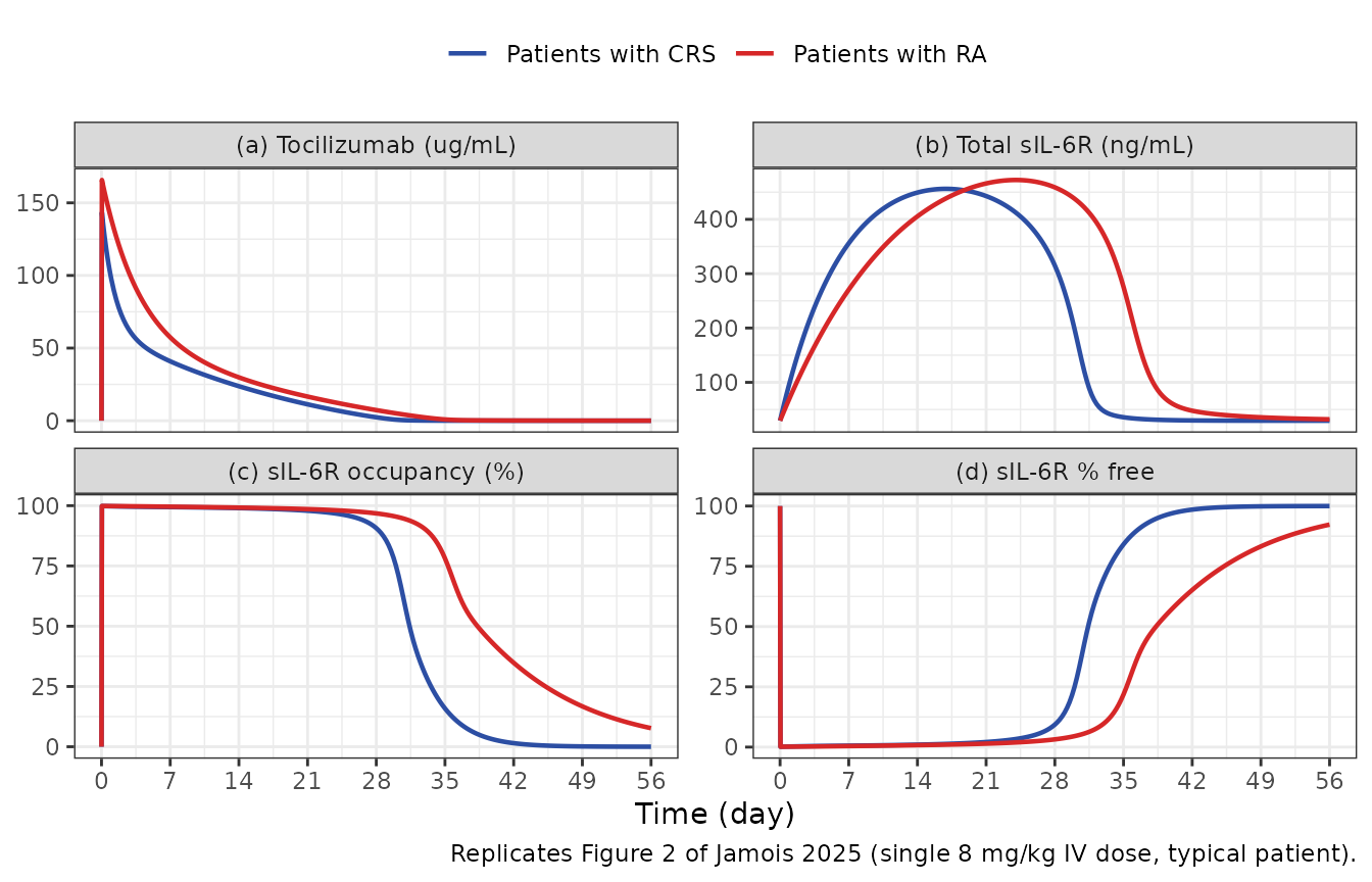
Figure 2(b) shows the total sIL-6R peak at about 455 ng/mL near day 17 for CRS and about 470 ng/mL near day 24 for RA (its axis label reads ug/mL, but the baseline near 30 identifies the unit as ng/mL, as in Table S4). The table below reads the same features from the simulation.
typ_feat <- sim_typ |>
  group_by(population) |>
  summarise(
    cmax = max(Cc),
    peak_total = max(total_target),
    t_peak_total = time[which.max(total_target)],
    ro_day28 = ro[time == 28],
    ro_day42 = ro[time == 42],
    .groups = "drop"
  )
typ_feat |>
  rename(
    "Population" = population,
    "Cmax (ug/mL)" = cmax,
    "Peak total sIL-6R (ng/mL)" = peak_total,
    "Time of peak (day)" = t_peak_total,
    "Occupancy day 28 (%)" = ro_day28,
    "Occupancy day 42 (%)" = ro_day42
  ) |>
knitr::kable(digits = 1, caption = "Typical-patient features (compare Figure 2).")| Population | Cmax (ug/mL) | Peak total sIL-6R (ng/mL) | Time of peak (day) | Occupancy day 28 (%) | Occupancy day 42 (%) |
|---|---|---|---|---|---|
| Patients with CRS | 143.3 | 456.2 | 17 | 90.7 | 1.5 |
| Patients with RA | 165.7 | 472.4 | 24 | 96.8 | 34.8 |
crs_feat <- typ_feat[typ_feat$population == "Patients with CRS", ]
ra_feat <- typ_feat[typ_feat$population == "Patients with RA", ]
stopifnot(
  # Figure 2(b): peaks about 455 (CRS) and 470 ng/mL (RA), CRS earlier.
  abs(crs_feat$peak_total / 455 - 1) < 0.1,
  abs(ra_feat$peak_total / 470 - 1) < 0.1,
  crs_feat$t_peak_total < ra_feat$t_peak_total - 3,
  # Figure 2(c): occupancy is lost earlier with CRS (higher CL).
  crs_feat$ro_day42 < 10,
  ra_feat$ro_day42 > 20
)
Virtual cohort (model-development studies)
Original data are not available. Covariates are drawn per study from the Table S4 means and SDs (log-normal for weight, creatinine clearance, HDL and baseline sIL-6R; normal for age), truncated to the observed ranges. HDL was 1.5 mmol/L for every NCT02500407 patient (Table S4: mean 1.5, SD 0, i.e. imputed at the reference). Every patient is given a first CRS event of grade >= 2 (see Assumptions).
rxode2::rxSetSeed(20250925)
set.seed(20250925)

rtrunc_lnorm <- function(n, mean, sd, lo, hi) {
  sdlog <- sqrt(log(1 + (sd / mean)^2))
  meanlog <- log(mean) - sdlog^2 / 2
  x <- rlnorm(n, meanlog, sdlog)
  pmin(pmax(x, lo), hi)
}
rtrunc_norm <- function(n, mean, sd, lo, hi) {
  pmin(pmax(rnorm(n, mean, sd), lo), hi)
}

# Table S4 summary statistics by study.
study_cov <- list(
  "NCT02500407 (mosunetuzumab)" = list(
    wt = c(84.4, 15.6, 66.2, 128), age = c(63.8, 10.1, 54, 87),
    crcl = c(90.1, 30.5, 44.5, 147), hdl = c(1.5, 0, 1.5, 1.5),
    sil6r = c(43.2, 26.5, 24.4, 82)
  ),
  "NCT03075696 (glofitamab)" = list(
    wt = c(72.6, 12.9, 53, 114), age = c(62.7, 13.8, 30, 85),
    crcl = c(79.6, 24.4, 33.4, 155), hdl = c(1.24, 0.42, 0.465, 2.5),
    sil6r = c(35.7, 20.1, 20.3, 103)
  )
)

make_subjects <- function(n, study, id_offset) {
  s <- study_cov[[study]]
  hdl <- if (s$hdl[2] == 0) rep(s$hdl[1], n) else do.call(rtrunc_lnorm, c(list(n), as.list(s$hdl)))
  data.frame(
    id = id_offset + seq_len(n),
    study = study,
    WT = do.call(rtrunc_lnorm, c(list(n), as.list(s$wt))),
    AGE = do.call(rtrunc_norm, c(list(n), as.list(s$age))),
    CRCL = do.call(rtrunc_lnorm, c(list(n), as.list(s$crcl))),
    HDLC = hdl,
    TSIL6R_BASE = do.call(rtrunc_lnorm, c(list(n), as.list(s$sil6r))),
    CRS_GRADE_GE2 = 1,
    STUDY_25220_28117 = 0,
    SC_INJ_GROUP3 = 0
  )
}

# 8 mg/kg (12 mg/kg below 30 kg), capped at 800 mg, 1-h IV infusion.
tcz_dose <- function(wt) pmin(ifelse(wt < 30, 12, 8) * wt, 800)

make_events <- function(subj, dose_times, obs_times) {
  doses <- subj |>
    tidyr::crossing(time = dose_times) |>
    mutate(amt = tcz_dose(WT), dur = 1 / 24, evid = 1L, cmt = "central")
  obs <- subj |>
    tidyr::crossing(time = obs_times) |>
    mutate(amt = 0, dur = 0, evid = 0L, cmt = "total_target")
  bind_rows(doses, obs) |> arrange(id, time, desc(evid))
}
Exposure and occupancy after 1-4 doses (Table S2 and Table 3)
Table S2 summarises individual (post hoc) exposures after one to four 8 mg/kg doses given 8 hours apart, by study. Each regimen arm below draws 100 virtual patients per study.
n_per_arm <- 100L
obs_s2 <- sort(unique(c(seq(0, 2, by = 1 / 24), seq(2, 28, by = 0.25))))
regimens <- 1:4
arms <- expand.grid(study = names(study_cov), n_doses = regimens, stringsAsFactors = FALSE)

events_s2 <- bind_rows(lapply(seq_len(nrow(arms)), function(i) {
  subj <- make_subjects(n_per_arm, arms$study[i], id_offset = (i - 1L) * n_per_arm)
  make_events(subj, dose_times = (seq_len(arms$n_doses[i]) - 1) * 8 / 24, obs_times = obs_s2) |>
    mutate(regimen = paste0(arms$n_doses[i], " x 8 mg/kg"))
}))
stopifnot(!anyDuplicated(unique(events_s2[, c("id", "time", "evid")])))

sim_s2 <- rxSolve(
  mod_crs,
  events = events_s2,
  keep = c("study", "regimen"),
  returnType = "data.frame"
)
#> ℹ parameter labels from comments will be replaced by 'label()'
conc_s2 <- sim_s2 |>
  filter(!is.na(Cc)) |>
  select(id, time, Cc, study, regimen) |>
  distinct(id, time, .keep_all = TRUE)
dose_s2 <- events_s2 |>
  filter(evid == 1) |>
  select(id, time, amt, study, regimen)

conc_obj <- PKNCAconc(conc_s2, Cc ~ time | study + regimen + id)
dose_obj <- PKNCAdose(dose_s2, amt ~ time | study + regimen + id)
intervals_s2 <- data.frame(
  start = c(0, 0, 0),
  end = c(28, 7, 28),
  cmax = c(TRUE, FALSE, FALSE),
  auclast = c(FALSE, TRUE, TRUE)
)
nca_s2 <- pk.nca(PKNCAdata(conc_obj, dose_obj, intervals = intervals_s2))

nca_s2_long <- as.data.frame(nca_s2$result) |>
  filter(PPTESTCD %in% c("cmax", "auclast")) |>
  mutate(interval = ifelse(PPTESTCD == "cmax", "Day 0-28", paste0("Day 0-", end))) |>
  select(study, regimen, interval, PPTESTCD, PPORRES)

# Table S2 medians.
published_s2 <- tibble::tribble(
  ~study, ~regimen, ~interval, ~PPTESTCD, ~PPORRES,
  "NCT02500407 (mosunetuzumab)", "1 x 8 mg/kg", "Day 0-28", "cmax", 131,
  "NCT02500407 (mosunetuzumab)", "2 x 8 mg/kg", "Day 0-28", "cmax", 246,
  "NCT02500407 (mosunetuzumab)", "3 x 8 mg/kg", "Day 0-28", "cmax", 349,
  "NCT02500407 (mosunetuzumab)", "4 x 8 mg/kg", "Day 0-28", "cmax", 441,
  "NCT03075696 (glofitamab)", "1 x 8 mg/kg", "Day 0-28", "cmax", 149,
  "NCT03075696 (glofitamab)", "2 x 8 mg/kg", "Day 0-28", "cmax", 281,
  "NCT03075696 (glofitamab)", "3 x 8 mg/kg", "Day 0-28", "cmax", 398,
  "NCT03075696 (glofitamab)", "4 x 8 mg/kg", "Day 0-28", "cmax", 502,
  "NCT02500407 (mosunetuzumab)", "1 x 8 mg/kg", "Day 0-7", "auclast", 447,
  "NCT02500407 (mosunetuzumab)", "2 x 8 mg/kg", "Day 0-7", "auclast", 909,
  "NCT02500407 (mosunetuzumab)", "3 x 8 mg/kg", "Day 0-7", "auclast", 1360,
  "NCT02500407 (mosunetuzumab)", "4 x 8 mg/kg", "Day 0-7", "auclast", 1790,
  "NCT03075696 (glofitamab)", "1 x 8 mg/kg", "Day 0-7", "auclast", 464,
  "NCT03075696 (glofitamab)", "2 x 8 mg/kg", "Day 0-7", "auclast", 940,
  "NCT03075696 (glofitamab)", "3 x 8 mg/kg", "Day 0-7", "auclast", 1400,
  "NCT03075696 (glofitamab)", "4 x 8 mg/kg", "Day 0-7", "auclast", 1850,
  "NCT02500407 (mosunetuzumab)", "1 x 8 mg/kg", "Day 0-28", "auclast", 676,
  "NCT02500407 (mosunetuzumab)", "2 x 8 mg/kg", "Day 0-28", "auclast", 1580,
  "NCT02500407 (mosunetuzumab)", "3 x 8 mg/kg", "Day 0-28", "auclast", 2490,
  "NCT02500407 (mosunetuzumab)", "4 x 8 mg/kg", "Day 0-28", "auclast", 3400,
  "NCT03075696 (glofitamab)", "1 x 8 mg/kg", "Day 0-28", "auclast", 915,
  "NCT03075696 (glofitamab)", "2 x 8 mg/kg", "Day 0-28", "auclast", 2100,
  "NCT03075696 (glofitamab)", "3 x 8 mg/kg", "Day 0-28", "auclast", 3290,
  "NCT03075696 (glofitamab)", "4 x 8 mg/kg", "Day 0-28", "auclast", 4460
)

cmp_s2 <- ncaComparisonTable(
  simulated = nca_s2_long,
  reference = published_s2,
  by = c("study", "regimen", "interval"),
  units = c(cmax = "ug/mL", auclast = "ug*day/mL"),
  tolerance_pct = 20
)
knitr::kable(
  cmp_s2,
  caption = paste(
    "Simulated (median of 100 virtual patients per arm) vs Table S2 medians.",
    attr(cmp_s2, "footnote")
  )
)| NCA parameter | study | regimen | interval | Reference | Simulated | % diff |
|---|---|---|---|---|---|---|
| Cmax (ug/mL) | NCT02500407 (mosunetuzumab) | 1 x 8 mg/kg | Day 0-28 | 131 | 151 | +15.0% |
| Cmax (ug/mL) | NCT02500407 (mosunetuzumab) | 2 x 8 mg/kg | Day 0-28 | 246 | 297 | +20.6%* |
| Cmax (ug/mL) | NCT02500407 (mosunetuzumab) | 3 x 8 mg/kg | Day 0-28 | 349 | 371 | +6.4% |
| Cmax (ug/mL) | NCT02500407 (mosunetuzumab) | 4 x 8 mg/kg | Day 0-28 | 441 | 487 | +10.5% |
| Cmax (ug/mL) | NCT03075696 (glofitamab) | 1 x 8 mg/kg | Day 0-28 | 149 | 150 | +0.7% |
| Cmax (ug/mL) | NCT03075696 (glofitamab) | 2 x 8 mg/kg | Day 0-28 | 281 | 270 | -3.9% |
| Cmax (ug/mL) | NCT03075696 (glofitamab) | 3 x 8 mg/kg | Day 0-28 | 398 | 366 | -8.0% |
| Cmax (ug/mL) | NCT03075696 (glofitamab) | 4 x 8 mg/kg | Day 0-28 | 502 | 478 | -4.8% |
| AUClast (ug*day/mL) | NCT02500407 (mosunetuzumab) | 1 x 8 mg/kg | Day 0-28 | 676 | 937 | +38.6%* |
| AUClast (ug*day/mL) | NCT02500407 (mosunetuzumab) | 1 x 8 mg/kg | Day 0-7 | 447 | 481 | +7.6% |
| AUClast (ug*day/mL) | NCT02500407 (mosunetuzumab) | 2 x 8 mg/kg | Day 0-28 | 1580 | 2090 | +32.0%* |
| AUClast (ug*day/mL) | NCT02500407 (mosunetuzumab) | 2 x 8 mg/kg | Day 0-7 | 909 | 979 | +7.7% |
| AUClast (ug*day/mL) | NCT02500407 (mosunetuzumab) | 3 x 8 mg/kg | Day 0-28 | 2490 | 3130 | +25.9%* |
| AUClast (ug*day/mL) | NCT02500407 (mosunetuzumab) | 3 x 8 mg/kg | Day 0-7 | 1360 | 1370 | +0.9% |
| AUClast (ug*day/mL) | NCT02500407 (mosunetuzumab) | 4 x 8 mg/kg | Day 0-28 | 3400 | 3980 | +17.1% |
| AUClast (ug*day/mL) | NCT02500407 (mosunetuzumab) | 4 x 8 mg/kg | Day 0-7 | 1790 | 1770 | -0.9% |
| AUClast (ug*day/mL) | NCT03075696 (glofitamab) | 1 x 8 mg/kg | Day 0-28 | 915 | 809 | -11.6% |
| AUClast (ug*day/mL) | NCT03075696 (glofitamab) | 1 x 8 mg/kg | Day 0-7 | 464 | 454 | -2.2% |
| AUClast (ug*day/mL) | NCT03075696 (glofitamab) | 2 x 8 mg/kg | Day 0-28 | 2100 | 1830 | -12.9% |
| AUClast (ug*day/mL) | NCT03075696 (glofitamab) | 2 x 8 mg/kg | Day 0-7 | 940 | 909 | -3.4% |
| AUClast (ug*day/mL) | NCT03075696 (glofitamab) | 3 x 8 mg/kg | Day 0-28 | 3290 | 2880 | -12.4% |
| AUClast (ug*day/mL) | NCT03075696 (glofitamab) | 3 x 8 mg/kg | Day 0-7 | 1400 | 1280 | -8.5% |
| AUClast (ug*day/mL) | NCT03075696 (glofitamab) | 4 x 8 mg/kg | Day 0-28 | 4460 | 3900 | -12.6% |
| AUClast (ug*day/mL) | NCT03075696 (glofitamab) | 4 x 8 mg/kg | Day 0-7 | 1850 | 1800 | -2.9% |
Table S2 also reports the concentration and the sIL-6R occupancy on days 7, 14, 21 and 28, and Table 3 pools the occupancy across both studies.
tp_sim <- sim_s2 |>
  filter(time %in% c(7, 14, 21, 28)) |>
  group_by(study, regimen, time) |>
  summarise(Cc = median(Cc), ro = median(ro), .groups = "drop")

tp_pub <- tibble::tribble(
  ~study, ~regimen, ~time, ~Cc_pub, ~ro_pub,
  "NCT02500407 (mosunetuzumab)", "1 x 8 mg/kg", 7, 32.3, 99.3,
  "NCT02500407 (mosunetuzumab)", "1 x 8 mg/kg", 14, 17.3, 98.6,
  "NCT02500407 (mosunetuzumab)", "1 x 8 mg/kg", 21, 8.23, 97.1,
  "NCT02500407 (mosunetuzumab)", "1 x 8 mg/kg", 28, 1.76, 86.2,
  "NCT02500407 (mosunetuzumab)", "2 x 8 mg/kg", 7, 72, 99.7,
  "NCT02500407 (mosunetuzumab)", "2 x 8 mg/kg", 14, 45.5, 99.5,
  "NCT02500407 (mosunetuzumab)", "2 x 8 mg/kg", 21, 30.1, 99.2,
  "NCT02500407 (mosunetuzumab)", "2 x 8 mg/kg", 28, 18.4, 98.7,
  "NCT03075696 (glofitamab)", "1 x 8 mg/kg", 7, 41.6, 99.4,
  "NCT03075696 (glofitamab)", "1 x 8 mg/kg", 14, 26.3, 99.1,
  "NCT03075696 (glofitamab)", "1 x 8 mg/kg", 21, 14.3, 98.3,
  "NCT03075696 (glofitamab)", "1 x 8 mg/kg", 28, 4.68, 95.1,
  "NCT03075696 (glofitamab)", "2 x 8 mg/kg", 7, 91.2, 99.7,
  "NCT03075696 (glofitamab)", "2 x 8 mg/kg", 14, 64, 99.6,
  "NCT03075696 (glofitamab)", "2 x 8 mg/kg", 21, 43.3, 99.4,
  "NCT03075696 (glofitamab)", "2 x 8 mg/kg", 28, 25.5, 99.1
)

tp_cmp <- inner_join(tp_pub, tp_sim, by = c("study", "regimen", "time"))
tp_cmp |>
  rename(
    "Study" = study, "Regimen" = regimen, "Day" = time,
    "Cc Table S2 (ug/mL)" = Cc_pub, "Cc simulated (ug/mL)" = Cc,
    "Occupancy Table S2 (%)" = ro_pub, "Occupancy simulated (%)" = ro
  ) |>
knitr::kable(digits = c(0, 0, 0, 2, 2, 1, 1), caption = "Median concentration and sIL-6R occupancy by day (Table S2).")| Study | Regimen | Day | Cc Table S2 (ug/mL) | Occupancy Table S2 (%) | Cc simulated (ug/mL) | Occupancy simulated (%) |
|---|---|---|---|---|---|---|
| NCT02500407 (mosunetuzumab) | 1 x 8 mg/kg | 7 | 32.30 | 99.3 | 43.4 | 99.4 |
| NCT02500407 (mosunetuzumab) | 1 x 8 mg/kg | 14 | 17.30 | 98.6 | 25.9 | 99.1 |
| NCT02500407 (mosunetuzumab) | 1 x 8 mg/kg | 21 | 8.23 | 97.1 | 13.7 | 98.3 |
| NCT02500407 (mosunetuzumab) | 1 x 8 mg/kg | 28 | 1.76 | 86.2 | 4.8 | 95.2 |
| NCT02500407 (mosunetuzumab) | 2 x 8 mg/kg | 7 | 72.00 | 99.7 | 90.4 | 99.7 |
| NCT02500407 (mosunetuzumab) | 2 x 8 mg/kg | 14 | 45.50 | 99.5 | 61.4 | 99.6 |
| NCT02500407 (mosunetuzumab) | 2 x 8 mg/kg | 21 | 30.10 | 99.2 | 37.2 | 99.4 |
| NCT02500407 (mosunetuzumab) | 2 x 8 mg/kg | 28 | 18.40 | 98.7 | 22.6 | 98.9 |
| NCT03075696 (glofitamab) | 1 x 8 mg/kg | 7 | 41.60 | 99.4 | 38.6 | 99.4 |
| NCT03075696 (glofitamab) | 1 x 8 mg/kg | 14 | 26.30 | 99.1 | 21.6 | 98.9 |
| NCT03075696 (glofitamab) | 1 x 8 mg/kg | 21 | 14.30 | 98.3 | 9.1 | 97.4 |
| NCT03075696 (glofitamab) | 1 x 8 mg/kg | 28 | 4.68 | 95.1 | 1.4 | 85.4 |
| NCT03075696 (glofitamab) | 2 x 8 mg/kg | 7 | 91.20 | 99.7 | 82.8 | 99.7 |
| NCT03075696 (glofitamab) | 2 x 8 mg/kg | 14 | 64.00 | 99.6 | 52.5 | 99.5 |
| NCT03075696 (glofitamab) | 2 x 8 mg/kg | 21 | 43.30 | 99.4 | 33.4 | 99.3 |
| NCT03075696 (glofitamab) | 2 x 8 mg/kg | 28 | 25.50 | 99.1 | 18.2 | 98.7 |
ro_pooled <- sim_s2 |>
  filter(time %in% c(14, 21), regimen %in% c("1 x 8 mg/kg", "2 x 8 mg/kg")) |>
  group_by(regimen, time) |>
  summarise(ro_median = median(ro), .groups = "drop")
knitr::kable(
  ro_pooled |> rename("Regimen" = regimen, "Day" = time, "Median occupancy (%)" = ro_median),
  digits = 1,
  caption = "Pooled median occupancy; Table 3 reports 99 / 98.2 % (1 dose, day 14 / 21) and 99.6 / 99.4 % (2 doses)."
)| Regimen | Day | Median occupancy (%) |
|---|---|---|
| 1 x 8 mg/kg | 14 | 99.0 |
| 1 x 8 mg/kg | 21 | 97.9 |
| 2 x 8 mg/kg | 14 | 99.6 |
| 2 x 8 mg/kg | 21 | 99.3 |
cmp_num <- nca_s2_long |>
  group_by(study, regimen, interval, PPTESTCD) |>
  summarise(sim = median(PPORRES), .groups = "drop") |>
  inner_join(published_s2, by = c("study", "regimen", "interval", "PPTESTCD")) |>
  mutate(pct_diff = 100 * (sim / PPORRES - 1))
early_pct <- cmp_num |>
  filter(PPTESTCD == "cmax" | interval == "Day 0-7") |>
  pull(pct_diff)
ro_pub_t3 <- c(99, 98.2, 99.6, 99.4) # Table 3: 1 dose day 14, 21; 2 doses day 14, 21
stopifnot(
  # Cmax and AUC0-7 are set by dose, VC and the first week of CL: a
  # mis-transcribed volume, dose or CRS factor moves the whole set by tens of
  # percent. Centre and a robust quantile, not the extremes (independent
  # 100-patient arms put single cells about 5-20% off).
  abs(median(early_pct)) < 10,
  quantile(abs(early_pct), 0.9) < 25,
  # Table 3 pooled median occupancy, to within 2 percentage points.
  all(abs(ro_pooled$ro_median - ro_pub_t3) < 2)
)
The simulated medians reproduce Cmax and AUC0-7 for both studies and all four regimens, and the pooled median occupancy of Table 3 to within half a percentage point. The 0-28-day AUC and the day-14 to day-28 concentrations are higher than Table S2 for the mosunetuzumab study and lower for the glofitamab study. The paper reports that the individual random effects on CL and VC were biased by study (higher CL and VC in NCT02500407 males) but kept no study effect in the model; the Table S2 values are post hoc individual estimates that carry that bias, while a simulation from the typical parameters cannot. The late tail also depends on the share of patients whose first CRS event was grade 1 (lower CL), which the paper does not report. These columns are shown for comparison and are not gated.
Repeat dosing over two cycles (Figure 3)
Figure 3 simulates the model-development patients receiving tocilizumab on days 0, 7, 42, 63 and 84, with (a) two doses 8 h apart on every occasion or (b) one dose on days 7 and 63, against the 649 ug/mL FDA safety threshold. The replication uses 61 virtual patients drawn in the study proportions.
obs_f3 <- sort(unique(c(seq(0, 98, by = 0.25), c(0, 7, 42, 63, 84) + 9 / 24)))
subj_f3 <- bind_rows(
  make_subjects(16, "NCT02500407 (mosunetuzumab)", id_offset = 0L),
  make_subjects(45, "NCT03075696 (glofitamab)", id_offset = 16L)
)
q8 <- 8 / 24
scen_a <- c(0, q8, 7, 7 + q8, 42, 42 + q8, 63, 63 + q8, 84, 84 + q8)
scen_b <- c(0, q8, 7, 42, 42 + q8, 63, 84, 84 + q8)
events_f3 <- bind_rows(
  make_events(subj_f3, scen_a, obs_f3) |> mutate(scenario = "(a) 2 doses on every occasion"),
  make_events(subj_f3 |> mutate(id = id + 100L), scen_b, obs_f3) |>
    mutate(scenario = "(b) 1 dose on days 7 and 63")
)
stopifnot(!anyDuplicated(unique(events_f3[, c("id", "time", "evid")])))

sim_f3 <- rxSolve(mod_crs, events = events_f3, keep = "scenario", returnType = "data.frame")

f3_long <- sim_f3 |>
  select(id, time, scenario, Cc, ro) |>
  pivot_longer(c(Cc, ro), names_to = "quantity") |>
  mutate(quantity = ifelse(quantity == "Cc", "Concentration (ug/mL)", "Receptor occupancy (%)"))

ggplot(f3_long, aes(time, value, group = id)) +
  geom_line(colour = "#2c4ea3", alpha = 0.4, linewidth = 0.3) +
  geom_hline(
    data = data.frame(
      quantity = c("Concentration (ug/mL)", "Receptor occupancy (%)"),
      y = c(649, 90),
      lt = c("dashed", "solid")
    ),
    aes(yintercept = y, linetype = lt), colour = "red"
  ) +
  scale_linetype_identity() +
  facet_grid(quantity ~ scenario, scales = "free_y") +
  scale_x_continuous(breaks = c(0, 7, 21, 42, 63, 84)) +
  labs(
    x = "Time (day)", y = NULL,
    caption = "Replicates Figure 3 of Jamois 2025 (61 virtual patients per scenario)."
  ) +
  theme_bw()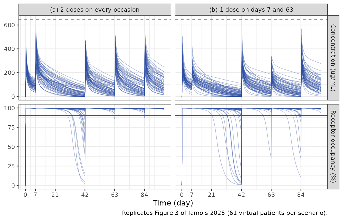
f3_summary <- sim_f3 |>
  group_by(scenario, id) |>
  summarise(cmax = max(Cc), .groups = "drop") |>
  group_by(scenario) |>
  summarise(
    median_cmax = median(cmax),
    p90_cmax = unname(quantile(cmax, 0.9)),
    .groups = "drop"
  )
knitr::kable(
  f3_summary |> rename("Scenario" = scenario, "Median Cmax (ug/mL)" = median_cmax, "90th percentile Cmax (ug/mL)" = p90_cmax),
  digits = 0
)| Scenario | Median Cmax (ug/mL) | 90th percentile Cmax (ug/mL) |
|---|---|---|
| (a) 2 doses on every occasion | 398 | 505 |
| (b) 1 dose on days 7 and 63 | 321 | 435 |
Assumptions and deviations
-
CRS grade. The paper does not report how many
model-development patients had a first CRS event of grade >= 2.
Tocilizumab was recommended for CRS of grade >= 2 and a missing grade
was imputed as 2 (Table S6), so every virtual patient is assigned
CRS_GRADE_GE2 = 1. Patients whose first event was grade 1 have 1.6-fold lower CL; including them would raise the late (day 21-28) concentrations. - Infusion duration. Not stated in the paper; a 1-hour IV infusion (the labelled duration) is assumed.
- Covariate distributions. Drawn from the Table S4 per-study means and SDs and truncated to the observed ranges; correlations between covariates are not reproduced. Albumin and total protein are not needed by the CRS model (their effects are fixed to 0).
- Typical patient in Figure 2. The figure does not give its covariates; the model reference values and a common baseline sIL-6R of 29.4 ng/mL are used for both populations.
- RA / JIA model structure. The paper publishes the NONMEM control stream only for the CRS model (Table S6). The RA / JIA model file reuses that structure with the CRS terms removed, the Table S1 albumin and total-protein effects restored, and the Table S1 random-effect structure (including a separate VP eta correlated with the VC eta); the population metadata are sparse because the paper does not describe the RA / JIA data set.
-
SC_INJ_GROUP3. Table S6 multiplies the log SC bioavailability by theta17 = 0.692 whenSINJ = 3(Table S1 ‘F SC,SJIT3’), but neither the paper nor the supplement definesSINJ. The maintainers kept the effect as an opaquely named indicator so it remains selectable; it has no effect on IV doses and is 0 throughout this article. -
Residual-error variability. The tocilizumab and
sIL-6R residual SDs carry between-subject random effects
(
etaruv,etaruv_total_target; Table S6EXP(ETA(13)),EXP(ETA(14))), encoded as the SD multiplier on the log-normal error. - Errata. The only post-publication change (23 August 2025) is to the copyright line; no parameter is affected.