Afatinib + HangAmDan-B1 tumor growth inhibition in HCC827-GR xenograft mice (Yang 2025)
Source:vignettes/articles/Yang_2025_afatinib_mouse.Rmd
Yang_2025_afatinib_mouse.RmdModel and source
Yang 2025 links a one-compartment oral PK model of afatinib (AFT) in
mice to a Simeoni tumor-growth-inhibition model of gefitinib-resistant
HCC827 (HCC827-GR) non-small-cell lung cancer xenografts. Natural growth
switches smoothly from exponential (rate lambda0) to linear (rate
lambda1); afatinib moves proliferating cells into a three-stage
damaged-cell chain at a rate proportional to its serum concentration
(potency KAFT). The herbal mixture HangAmDan-B1 (HAD-B1) has no PK
component (its constituents were not detectable in serum); it enters as
a binary indicator that multiplies afatinib potency by
1 + alpha_syn.
The paper fits natural growth to the vehicle-control group first, then fixes lambda0 and lambda1 and fits the pooled afatinib and combination groups for the final PK/PD model (Table 3, “Treated Groups”). The file carries that final model.
ui <- rxode2::rxode(readModelDb("Yang_2025_afatinib_mouse"))
#> ℹ parameter labels from comments will be replaced by 'label()'
tv <- rxode2::zeroRe(ui)- Citation: Yang SY, Ngo LT, Lee S, Yun HY, Bui TT, Kim DH, Chae JW, Park S. Model-Based Evaluation of HangAmDan-B1 and Afatinib Combination Therapy in HCC827 Xenograft Mice with Resistance to Epidermal Growth Factor Receptor Tyrosine Kinase Inhibitor. Pharmaceuticals (Basel). 2025;18(5):748. doi:10.3390/ph18050748.
- Article (open access): https://doi.org/10.3390/ph18050748
- Supplement:
pharmaceuticals-3591387-supplementary.pdf(bioanalytical method, PK and PK/PD goodness-of-fit plots, HAD-B1 HPLC profile). It holds no additional parameter values or control streams. - Tumor-growth data: Song et al. 2022 (reference 12 of Yang 2025).
Crossref lists no correction or erratum for this article (checked 2026-11-04).
Population
PK was measured in tumor-free female BALB/c nude mice (5 weeks old, 18-20 g; n = 6 per arm) given afatinib 10 mg/kg once daily by oral gavage for 30 days, alone or with HAD-B1 400 mg/kg once daily; serum was sampled 0.5, 2, 4 and 8 h after the day-30 dose (Section 4.2.2). The tumor data come from BALB/c nude mice inoculated subcutaneously with 1e6 HCC827-GR cells, randomised at 80-100 mm^3 (n = 6 per group) to vehicle, afatinib 10 mg/kg/day, HAD-B1 400 mg/kg/day, or both, for 30 days. For model fitting the authors generated 100 tumor-growth profiles per group from the published group mean and SD (Section 4.3.1).
pop <- ui$population
tibble::tibble(
  Field = names(pop),
  Value = vapply(pop, function(x) paste(x, collapse = "; "), character(1))
) |>
knitr::kable()| Field | Value |
|---|---|
| species | mouse (BALB/c nude; PK in tumor-free females, tumor growth with subcutaneous gefitinib-resistant HCC827 xenograft) |
| n_subjects | 36 |
| n_studies | 2 |
| age_range | 5 weeks at purchase (PK mice) |
| weight_range | 18-20 g at purchase (PK mice) |
| sex_female_pct | NA |
| race_ethnicity | NA |
| disease_state | PK: tumor-free mice. PD: subcutaneous right-flank xenograft of gefitinib-resistant HCC827 human non-small-cell lung cancer cells (HCC827-GR; 1e6 cells), randomised at 80-100 mm^3. |
| dose_range | Afatinib 10 mg/kg orally once daily for 30 days, alone or with HAD-B1 400 mg/kg orally once daily; tumor study also had vehicle-control and HAD-B1-alone arms. |
| regions | Republic of Korea (preclinical) |
| notes | PK: n = 6 female BALB/c nude mice per arm (afatinib alone, afatinib + HAD-B1), serum sampled 0.5, 2, 4 and 8 h after the day-30 dose (Section 4.2.2). PD: tumor-volume data from Song et al. 2022 (n = 6 mice per group: vehicle, afatinib, HAD-B1, afatinib + HAD-B1); for modeling, 100 tumor-growth profiles per group were generated from the published group mean and SD assuming normality (Section 4.3.1). Natural growth was fitted to the control group first; lambda0 and lambda1 were then fixed and the treated groups were pooled for the final PK/PD fit (Table 3, ‘Treated Groups’), which is the parameter set encoded here. |
Source trace
Every ini() value carries an in-file comment naming its
source.
| Parameter | Value | Source |
|---|---|---|
lka (Ka) |
0.2 1/h | Table 2 |
lcl (CL/F) |
24.5 L/h/kg | Table 2 |
lvc (Vd/F) |
56.1 L/kg | Table 2 |
etalcl, etalvc
|
30.9%, 50.2% CV -> log(1 + CV^2) | Table 2 |
propSd (afatinib) |
0.29 | Table 2, Prop.ER 29.0% |
ltumorExpGrowth (lambda0), fixed |
0.156 1/day | Table 3 |
ltumorLinGrowth (lambda1), fixed |
34.9 mm^3/day | Table 3 (prose: 35.5; see Assumptions) |
psi (phi), fixed |
20 | Table 3; Section 4.3.2 |
lrbase_tumor (V0) |
32.7 mm^3 | Table 3, Treated Groups |
ldamageTransit (K1) |
2.2 1/day | Table 3, Treated Groups |
ldrugSlope (KAFT) |
0.0034 mL/ng/day | Table 3, Treated Groups |
e_conmed_hadb1_drugSlope (alpha_syn) |
0.45 | Table 3, Treated Groups; Equation 1 |
propSd_tumor_vol |
0.215 | Table 3, Treated Groups Prop.ER |
| One-compartment first-order absorption PK | – | Equations 2-3 |
| Smooth exponential-to-linear growth, kill term, transit chain | – | Equations 8, 10-16 |
| Treatment start at day 7 after inoculation | – | Section 4.3.2 |
Model time is days. Table 2 prints Ka in 1/h and CL/F in L/h/kg;
model() multiplies both by 24. Doses are in mg/kg and
volumes in L/kg, so Cc = 1000 * central / vc is in ng/mL,
the scale of KAFT.
Afatinib PK at steady state (Figure 2, Table 1)
The PK study dosed 10 mg/kg once daily for 30 days and sampled after
the last dose. A cohort of 100 virtual mice per arm is simulated; the
HAD-B1 indicator does not enter the PK, so the two arms differ only by
sampling noise. The observation rows carry dvid = 1
(afatinib) because both declared endpoints are algebraic
observables.
n_pk <- 100L
pk_hours <- sort(unique(c(0, 0.5, 2, 4, 8, seq(0, 24, by = 0.25))))
pk_events <- function(id0, hadb1) {
  ids <- id0 + seq_len(n_pk) - 1L
  doses <- tidyr::expand_grid(id = ids, time = 0:29) |>
    dplyr::mutate(evid = 1L, amt = 10, cmt = "depot", dvid = NA_integer_)
  obs <- tidyr::expand_grid(id = ids, time = 29 + pk_hours / 24) |>
    dplyr::mutate(evid = 0L, amt = 0, cmt = NA_character_, dvid = 1L)
  dplyr::bind_rows(doses, obs) |>
    dplyr::arrange(id, time, dplyr::desc(evid)) |>
    dplyr::mutate(CONMED_HADB1 = hadb1)
}
ev_pk <- dplyr::bind_rows(pk_events(1L, 0), pk_events(n_pk + 1L, 1))
rxode2::rxSetSeed(20251)
sim_pk <- as.data.frame(rxode2::rxSolve(ui, ev_pk, returnType = "data.frame", keep = "CONMED_HADB1")) |>
  dplyr::mutate(
    treatment = ifelse(CONMED_HADB1 == 1, "AFT + HAD-B1", "AFT"),
    tad_h = round((time - 29) * 24, 4)
  )
sim_pk |>
  dplyr::filter(tad_h <= 8) |>
  dplyr::group_by(treatment, tad_h) |>
  dplyr::summarise(
    p05 = quantile(sim, 0.05), p50 = median(sim), p95 = quantile(sim, 0.95),
    .groups = "drop"
  ) |>
  ggplot(aes(tad_h, p50)) +
  geom_ribbon(aes(ymin = p05, ymax = p95), fill = "steelblue", alpha = 0.3) +
  geom_line() +
  facet_wrap(~treatment) +
  labs(x = "Time after the day-30 dose (h)", y = "Afatinib (ng/mL)")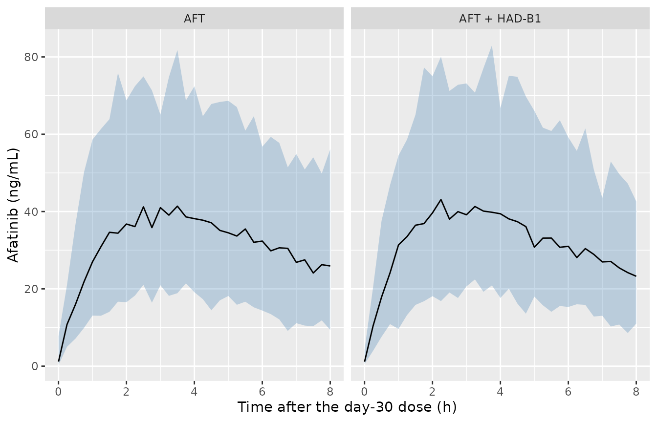
Simulated afatinib serum concentration after the day-30 dose (median and 90% prediction interval including residual error). Replicates the layout of Figure 2 of Yang 2025.
NCA
The published NCA used the four sampling times (0.5, 2, 4, 8 h) of the day-30 profile; AUClst,ss is therefore AUC from the dose to 8 h. The simulated NCA uses the same times plus a pre-dose sample, on the individual predictions.
conc_nca <- sim_pk |>
  dplyr::filter(tad_h %in% c(0, 0.5, 2, 4, 8)) |>
  dplyr::filter(!is.na(Cc)) |>
  dplyr::select(id, treatment, tad_h, Cc)
dose_nca <- conc_nca |>
  dplyr::distinct(id, treatment) |>
  dplyr::mutate(tad_h = 0, dose = 10)
o_conc <- PKNCA::PKNCAconc(conc_nca, Cc ~ tad_h | treatment + id)
o_dose <- PKNCA::PKNCAdose(dose_nca, dose ~ tad_h | treatment + id)
intervals <- data.frame(start = 0, end = 8, cmax = TRUE, auclast = TRUE)
nca_res <- PKNCA::pk.nca(PKNCA::PKNCAdata(o_conc, o_dose, intervals = intervals))
Yang 2025 Table 1 reports arithmetic means, so the simulated values are summarised by arm as arithmetic means before comparison.
sim_mean <- as.data.frame(nca_res) |>
  dplyr::filter(PPTESTCD %in% c("cmax", "auclast")) |>
  dplyr::group_by(treatment, PPTESTCD) |>
  dplyr::summarise(PPORRES = mean(PPORRES), .groups = "drop")
published <- tibble::tibble(
  treatment = c("AFT", "AFT + HAD-B1"),
  cmax = c(50.37, 48.50),
  auclast = c(287.63, 263.87)
)
cmp_nca <- nlmixr2lib::ncaComparisonTable(
  simulated = sim_mean,
  reference = published,
  by = "treatment",
  units = c(cmax = "ng/mL", auclast = "h*ng/mL"),
  tolerance_pct = 20
)
knitr::kable(cmp_nca, caption = "Simulated (mean of 100 mice per arm) vs Yang 2025 Table 1 (mean of 6 mice per arm). * differs from the reference by >20%.")| NCA parameter | treatment | Reference | Simulated | % diff |
|---|---|---|---|---|
| Cmax (ng/mL) | AFT | 50.4 | 43.2 | -14.2% |
| Cmax (ng/mL) | AFT + HAD-B1 | 48.5 | 44.1 | -9.0% |
| AUClast (h*ng/mL) | AFT | 288 | 262 | -8.7% |
| AUClast (h*ng/mL) | AFT + HAD-B1 | 264 | 264 | +0.2% |
pd <- as.numeric(gsub("[^0-9.+-]", "", cmp_nca$`% diff`))
# A clearance or volume off by the h-to-day factor, or a mg-to-ng slip, moves
# both quantities by an order of magnitude; the published means come from six
# mice per arm.
stopifnot(abs(median(pd)) < 25, max(abs(pd)) < 40)
The typical-value peak is lower than the observed mean (Cmax about 43 ng/mL at 3.3 h for a mouse with typical CL/F and Vd/F), which the inter-animal variability on CL/F and Vd/F partly closes in the cohort mean.
Tumor growth (Figure 5)
Figure 5 simulates the typical vehicle, afatinib and combination trajectories from inoculation, with treatment from day 7 and a 350 mm^3 threshold. All three curves start at the treated-groups V0 of 32.7 mm^3. The paper reports the threshold is reached on days 16, 22 and 28.
tumor_events <- function(id, treated, hadb1, by = 0.01) {
  obs <- data.frame(
    id = id, time = seq(0, 35, by = by), evid = 0L, amt = 0,
    cmt = NA_character_, dvid = 2L
  )
  doses <- if (treated) {
    data.frame(id = id, time = 7:36, evid = 1L, amt = 10, cmt = "depot", dvid = NA_integer_)
  } else {
    NULL
  }
  dplyr::bind_rows(doses, obs) |>
    dplyr::arrange(time, dplyr::desc(evid)) |>
    dplyr::mutate(CONMED_HADB1 = hadb1)
}
arms <- c("Control", "AFT", "COMB")
ev_tv <- dplyr::bind_rows(
  tumor_events(1L, FALSE, 0),
  tumor_events(2L, TRUE, 0),
  tumor_events(3L, TRUE, 1)
)
sim_tv <- as.data.frame(rxode2::rxSolve(tv, ev_tv, returnType = "data.frame")) |>
  dplyr::mutate(arm = factor(arms[id], levels = arms))
#> ℹ omega/sigma items treated as zero: 'etalcl', 'etalvc'
#> Warning: multi-subject simulation without without 'omega'

t350 <- sim_tv |>
  dplyr::group_by(arm) |>
  dplyr::summarise(
    `Simulated day` = min(time[tumor_vol >= 350]),
    `Volume at day 35 (mm^3)` = tumor_vol[time == 35],
    .groups = "drop"
  ) |>
  dplyr::mutate(`Yang 2025 day` = c(16, 22, 28), .after = arm)
knitr::kable(t350, digits = 1, caption = "Days to reach 350 mm^3 (typical values) vs Yang 2025 Section 2.2.3.")| arm | Yang 2025 day | Simulated day | Volume at day 35 (mm^3) |
|---|---|---|---|
| Control | 16 | 16.0 | 1014.1 |
| AFT | 22 | 21.1 | 516.6 |
| COMB | 28 | 26.5 | 407.7 |
ggplot(sim_tv, aes(time, tumor_vol, colour = arm)) +
  geom_line(linewidth = 1, linetype = "dashed") +
  geom_hline(yintercept = 350, colour = "red") +
  geom_vline(xintercept = 7, linetype = "dotted") +
  labs(x = "Time after inoculation (day)", y = "Tumor volume (mm^3)", colour = NULL)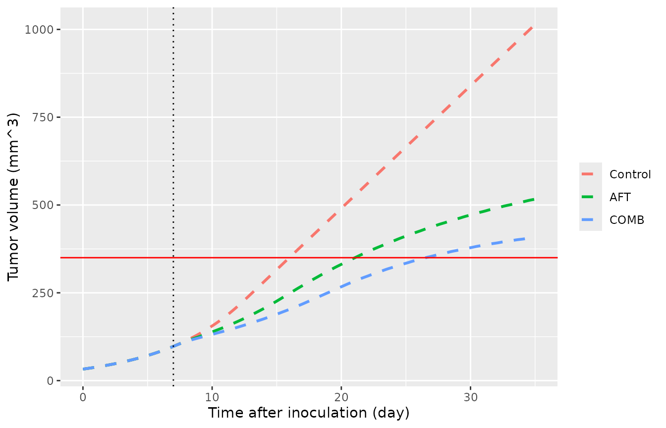
Typical-value tumor volume by arm. Replicates Figure 5 of Yang 2025; the red line is the 350 mm^3 threshold.
# Typical-value solve, so no sampling noise. A potency, transit or growth rate
# mis-transcribed by a factor of two moves the treated threshold days by more
# than three days.
stopifnot(all(abs(t350$`Simulated day` - t350$`Yang 2025 day`) <= 2))
The vehicle arm reaches the threshold on the published day; the treated arms reach it about one day (afatinib) and 1.5 days (combination) earlier than Figure 5. The digitised day-35 volumes of Figure 5 (about 960, 500 and 395 mm^3) sit within 6% of the simulated values.
Threshold concentration
Section 2.2.1 derives the concentration at which the kill rate matches exponential growth, CT = lambda0 / KAFT = 46 ng/mL, and Section 3 notes the observed average steady-state concentration (12 ng/mL) lies below it, so afatinib 10 mg/kg/day cannot eradicate the tumor.
th <- ui$theta
ct_aft <- exp(th[["ltumorExpGrowth"]]) / exp(th[["ldrugSlope"]])
ct_comb <- ct_aft / (1 + th[["e_conmed_hadb1_drugSlope"]])
cavg_ss <- 1000 * 10 / (exp(th[["lcl"]]) * 24) # ng/mL; dose / (CL/F * tau)
c(CT_AFT = ct_aft, CT_COMB = ct_comb, Cavg_ss_typical = cavg_ss)
#>          CT_AFT         CT_COMB Cavg_ss_typical
#>        45.88235        31.64300        17.00680
stopifnot(abs(ct_aft - 46) < 0.5)
The typical average steady-state concentration (dose / (CL/F x 24 h) = 17 ng/mL) is above the paper’s 12 ng/mL, which divides the 0-8 h AUClst,ss by the 24 h interval and so omits the 8-24 h tail; both are well below CT.
Tumor VPC (Figure 4)
A cohort of 100 mice per arm, each with its own afatinib PK, simulated with the tumor-volume residual error. The tumor model itself carries no inter-animal variability (Table 3), so the spread is residual error plus the PK variability propagated through the kill term.
n_tum <- 100L
ev_vpc <- dplyr::bind_rows(lapply(seq_along(arms), function(a) {
  dplyr::bind_rows(lapply(seq_len(n_tum), function(i) {
    tumor_events((a - 1L) * n_tum + i, a > 1, as.numeric(a == 3), by = 0.5)
  }))
}))
rxode2::rxSetSeed(20252)
sim_vpc <- as.data.frame(rxode2::rxSolve(ui, ev_vpc, returnType = "data.frame")) |>
  dplyr::mutate(arm = factor(arms[(id - 1L) %/% n_tum + 1L], levels = arms))
vpc_sum <- sim_vpc |>
  dplyr::filter(time >= 7) |>
  dplyr::group_by(arm, time) |>
  dplyr::summarise(
    p05 = quantile(sim, 0.05), p50 = median(sim), p95 = quantile(sim, 0.95),
    .groups = "drop"
  )
ggplot(vpc_sum, aes(time, p50)) +
  geom_ribbon(aes(ymin = p05, ymax = p95), fill = "steelblue", alpha = 0.3) +
  geom_line(colour = "darkred") +
  facet_wrap(~arm) +
  labs(x = "Time after inoculation (day)", y = "Tumor volume (mm^3)")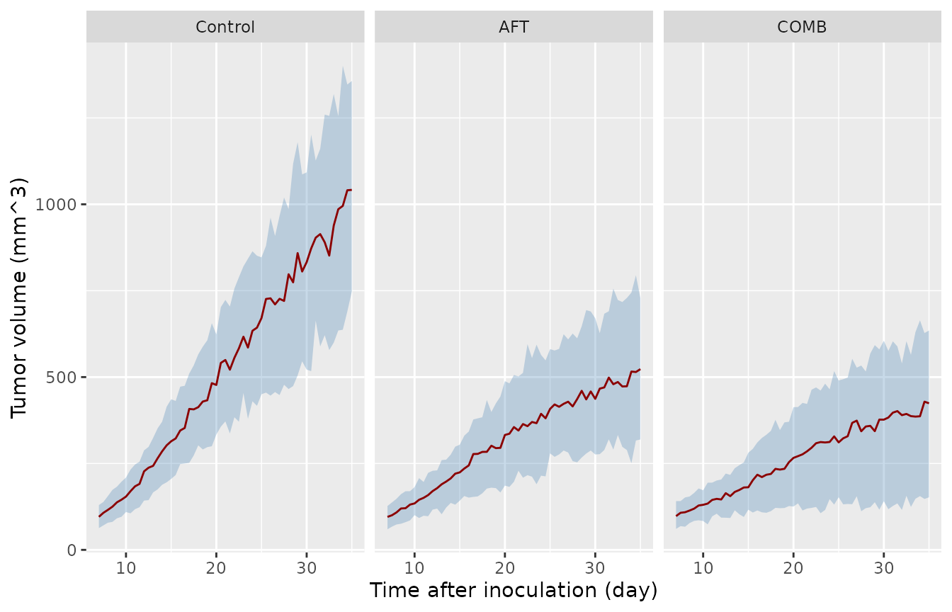
Simulated tumor volume (median and 90% prediction interval) by arm from treatment start. Compare with Figure 4 of Yang 2025.
day35 <- vpc_sum |> dplyr::filter(time == 35)
day35
#> # A tibble: 3 × 5
#>   arm      time   p05   p50   p95
#>   <fct>   <dbl> <dbl> <dbl> <dbl>
#> 1 Control    35  748. 1042. 1357.
#> 2 AFT        35  319.  523.  728.
#> 3 COMB       35  152.  424.  635.
# Median ordering at day 35 is driven by a 2-fold control/AFT gap and a 25%
# AFT/COMB gap in the typical values, far outside the median's sampling error.
stopifnot(
  day35$p50[day35$arm == "Control"] > day35$p50[day35$arm == "AFT"],
  day35$p50[day35$arm == "AFT"] > day35$p50[day35$arm == "COMB"]
)
The control panel of Figure 4 is the separate natural-growth fit (V0 = 21.4 mm^3, residual 0.169), so its curve here starts higher than the published one; see the first assumption below.
Assumptions and deviations
-
Control-group fit. Table 3 reports two columns. The
“Control Group” natural-growth fit (V0 = 21.4 mm^3, proportional
residual 0.169) supplied the fixed lambda0 and lambda1; the “Treated
Groups” fit is the final PK/PD model and is what the file carries (V0 =
32.7 mm^3, residual 0.215). Figure 5 uses V0 = 32.7 mm^3 for all three
arms. To reproduce the control-only fit (Figure 4A), override
lrbase_tumor = log(21.4)andpropSd_tumor_vol = 0.169. - lambda1. Table 3 prints 34.9 mm^3/day for both columns; the Results prose (Section 2.2.1) prints 35.5. The table value is used. Using 35.5 instead moves the threshold days by at most 0.3 day.
- Growth-switch term. Equations 8 and 10 apply the exponential-to-linear switch to the proliferating pool X1(t), consistent with the threshold definition in Equations 4-5; Simeoni 2004 applies it to total tumor volume. The printed form is encoded. The total-volume form gives threshold days of 16.0, 21.9 and 30.1 (vs 16.0, 21.1 and 26.5 here; published 16, 22 and 28), so Figure 5 does not separate the two.
- IIV scale. Table 2 prints IIV as percentages without a formula; they are read as CVs and converted with omega^2 = log(1 + CV^2) (0.0912 and 0.2247). Reading them as 100 x omega would give 0.0955 and 0.2520.
- Treatment start. Section 4.3.2 places treatment start at day 7 after inoculation; 30 daily doses (days 7-36) are simulated. The Figure 5 arrow is drawn nearer day 8.5; starting on day 8 moves the treated threshold days by about one day earlier, not later.
- PK in the tumor fit. The PK model was fitted to tumor-free mice and the tumor fit used simulated afatinib concentrations. In this file each simulated mouse carries its own PK random effects, which drive its tumor response.
- No inter-animal variability on tumor parameters. Table 3 reports none; the fit used 100 synthetic profiles per group generated from published group means and SDs.
-
HAD-B1. Estimated at one dose (400 mg/kg/day), with
no PK and no effect on afatinib exposure;
CONMED_HADB1has no dose dimension, and the HAD-B1 monotherapy arm of the tumor study (minimal suppression, not modelled) is equivalent to the control arm in this model.