Blinatumomab (Clements 2020)
Source:vignettes/articles/Clements_2020_blinatumomab.Rmd
Clements_2020_blinatumomab.RmdModel and source
mod <- rxode2::rxode(readModelDb("Clements_2020_blinatumomab"))
#> ℹ parameter labels from comments will be replaced by 'label()'- Citation: Clements JD, Zhu M, Kuchimanchi M, Terminello B, Doshi S. (2020). Population Pharmacokinetics of Blinatumomab in Pediatric and Adult Patients with Hematological Malignancies. Clinical Pharmacokinetics 59(4):463-474. doi:10.1007/s40262-019-00823-8.
- Article: https://doi.org/10.1007/s40262-019-00823-8
- PMC full text: https://www.ncbi.nlm.nih.gov/pmc/articles/PMC7109194/
One-compartment population PK model with linear first-order elimination for continuous intravenous blinatumomab (CD19/CD3 bispecific T cell engager) in pediatric and adult patients with hematological malignancies (Clements 2020). Fit by NONMEM 7.2 FOCE to serum concentrations from 674 patients (628 adults, 46 children aged 7 months to 16 years) pooled from eight phase I-III studies in relapsed/refractory B-precursor ALL (Philadelphia-negative and -positive), MRD-positive B-lineage ALL and relapsed NHL. Typical CL is 2.22 L/h and V 5.98 L at the reference body surface area of 1.876 m2; body surface area enters CL as a power function (exponent 0.620). Inter-individual variability is carried on CL only; the residual error is additive on the natural-log scale (transform-both-sides) and itself carries inter-individual variability on its magnitude.
Blinatumomab is given as a continuous intravenous (cIV) infusion over 4 weeks per cycle, either as a BSA-based dose (5 or 15 ug/m2/day) or as a fixed dose (9 or 28 ug/day). The US label uses the BSA-based dose below 45 kg and the fixed dose at or above 45 kg; the paper’s simulations were designed to support that cut-off.
Population
The analysis pooled 674 patients from eight studies (one phase I, one phase I/II, five phase II, one phase III; Table 1): 628 adults and 46 children aged 7 months to 16 years (study MT103-205). Diseases were relapsed/refractory Philadelphia-negative B-precursor ALL (472 adults, 46 children), relapsed/refractory Philadelphia-positive ALL (37), MRD-positive B-lineage ALL (52) and relapsed non-Hodgkin lymphoma (67). Median age 41.0 years (range 0.6-80), median weight 70.7 kg (7.5-149), median BSA 1.8 m2 (0.37-2.70); 39.7 % female and 85.9 % White (Results 3.1; Electronic Supplementary Material [ESM] Tables 1-2). Median creatinine clearance was 121 mL/min (36-150).
Source trace
| Element | Value | Source location |
|---|---|---|
| Structure: one compartment, linear first-order elimination, cIV input | – | Abstract; Results 3.3 |
lcl |
CL = 2.22 L/h | Table 3 |
lvc |
V = 5.98 L | Table 3 |
e_bsa_cl |
0.620 | Table 3 |
BSA covariate form CL * (BSA/1.876)^theta
|
reference 1.876 m2 | Table 3 footnote a |
etalcl |
47.6 %CV -> variance 0.476^2 | Table 3; ESM ‘Pharmacostatistical Modeling’ (%CV expressed approximately) |
| No IIV on V | – | Results 3.3 (‘an exponential IIV term was estimated for CL’) |
expSd |
55.9 %CV -> log-scale SD 0.559 | Table 3; ESM (transform-both-sides additive error) |
etaexpSd |
64.3 %CV -> variance 0.643^2 | Table 3 row ‘omega EPS’; Results 3.3 (‘additive error model in the log-domain with IIV’) |
| Concentration unit pg/mL | – | Methods 2.2 (assay LLOQ 50-100 pg/mL) |
Closed-form checks against the paper’s own derived numbers
The Discussion quotes the CL change at the extremes of BSA and the
typical half-life at four BSA values. These use only the typical
parameters, so they are exact checks of lcl,
lvc, e_bsa_cl and the 1.876 m2 reference.
cl_ref <- exp(mod$theta[["lcl"]])
vc_ref <- exp(mod$theta[["lvc"]])
e_bsa <- mod$theta[["e_bsa_cl"]]

bsa <- c(0.37, 1.31, 1.88, 2.7)
cl_i <- cl_ref * (bsa / 1.876)^e_bsa
closed <- data.frame(
  BSA = bsa,
  cl_change_pct = 100 * (cl_i / cl_ref - 1),
  paper_cl_change_pct = c(-63, -20, 0, 25),
  thalf_h = log(2) * vc_ref / cl_i,
  paper_thalf_h = c(5.11, 2.34, 1.86, 1.49)
)
closed |>
  dplyr::mutate(dplyr::across(-BSA, ~ signif(.x, 3))) |>
  dplyr::rename(
    "BSA (m2)" = BSA,
    "CL change, model (%)" = cl_change_pct,
    "CL change, paper (%)" = paper_cl_change_pct,
    "t1/2, model (h)" = thalf_h,
    "t1/2, paper (h)" = paper_thalf_h
  ) |>
knitr::kable(caption = "Typical CL change versus BSA 1.88 m2 and typical half-life (Discussion, paragraphs 3 and 4).")| BSA (m2) | CL change, model (%) | CL change, paper (%) | t1/2, model (h) | t1/2, paper (h) |
|---|---|---|---|---|
| 0.37 | -63.500 | -63 | 5.11 | 5.11 |
| 1.31 | -20.000 | -20 | 2.33 | 2.34 |
| 1.88 | 0.132 | 0 | 1.86 | 1.86 |
| 2.70 | 25.300 | 25 | 1.49 | 1.49 |
stopifnot(
  all(abs(closed$cl_change_pct - closed$paper_cl_change_pct) < 1),
  all(abs(closed$thalf_h - closed$paper_thalf_h) < 0.02)
)
All eight derived numbers are reproduced to the printed precision.
Virtual cohort
Table 2 of the paper summarises the non-compartmental (NCA) results in two body weight groups, 45 kg and above versus below 45 kg, for each cycle-1 dose. The cohort below reproduces those two groups. Below 45 kg the two dose types come from different patients: the only pediatric study (MT103-205) used BSA-based doses, so the patients below 45 kg who received a fixed dose were light adults from the fixed-dose studies (minimum weights 39 and 42 kg in studies 00103311 and 20120216, ESM Table 1). Body weight is therefore drawn as follows: 45 kg and above, log-normal with median 71 kg truncated at 45-149 kg; below 45 kg on a BSA-based dose, log-normal with median 21 kg (the MT103-205 median) truncated at 7.5-44.9 kg; below 45 kg on a fixed dose, uniform on 39-44.9 kg. BSA is derived from weight with the weight-only Livingston-Scott formula (BSA = 0.1173 x WT^0.6466), because the paper does not report heights. Each weight group receives each of the four cycle-1 doses, 100 subjects per arm.
rxode2::rxSetSeed(20200401)
n_per_arm <- 100

draw_wt <- function(n, median, lo, hi) {
  wt <- exp(rnorm(4 * n, log(median), 0.35))
  wt <- wt[wt >= lo & wt <= hi]
  wt[seq_len(n)]
}
bsa_ls <- function(wt) 0.1173 * wt^0.6466

arms <- expand.grid(
  wtgrp = c(">=45 kg", "<45 kg"),
  dose = c("9 ug/day", "28 ug/day", "5 ug/m2/day", "15 ug/m2/day"),
  stringsAsFactors = FALSE
)
arms$arm <- paste(arms$wtgrp, arms$dose, sep = ", ")

cohort <- do.call(rbind, lapply(seq_len(nrow(arms)), function(i) {
  heavy <- arms$wtgrp[i] == ">=45 kg"
  fixed_dose <- grepl("ug/day", arms$dose[i], fixed = TRUE) && !grepl("m2", arms$dose[i], fixed = TRUE)
  wt <- if (heavy) {
    draw_wt(n_per_arm, 71, 45, 149)
  } else if (fixed_dose) {
    runif(n_per_arm, 39, 44.9)
  } else {
    draw_wt(n_per_arm, 21, 7.5, 44.9)
  }
  data.frame(arm = arms$arm[i], wtgrp = arms$wtgrp[i], dose = arms$dose[i], WT = wt, BSA = bsa_ls(wt))
}))
cohort$id <- seq_len(nrow(cohort))
cohort$daily_ug <- with(cohort, dplyr::case_when(
  dose == "9 ug/day" ~ 9,
  dose == "28 ug/day" ~ 28,
  dose == "5 ug/m2/day" ~ 5 * BSA,
  dose == "15 ug/m2/day" ~ 15 * BSA
))
cohort |>
  dplyr::group_by(wtgrp) |>
  dplyr::summarise(
    n = dplyr::n(),
    WT_median = median(WT),
    BSA_median = median(BSA),
    BSA_min = min(BSA),
    BSA_max = max(BSA)
  ) |>
knitr::kable(digits = 2, caption = "Virtual cohort body size by weight group.")| wtgrp | n | WT_median | BSA_median | BSA_min | BSA_max |
|---|---|---|---|---|---|
| <45 kg | 400 | 39.12 | 1.26 | 0.44 | 1.37 |
| >=45 kg | 400 | 73.76 | 1.89 | 1.38 | 2.97 |
Simulation
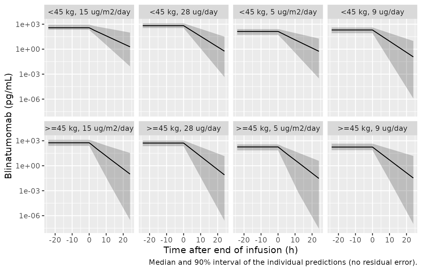
Each subject receives a 7-day continuous infusion (the cycle-1 step
duration), sampled densely over the last day of infusion and for 24 h
after the infusion stops. Observation rows are on the
central compartment; Cc (pg/mL) is returned
alongside.
inf_h <- 168
obs_t <- sort(unique(c(0, seq(144, inf_h, by = 2), inf_h + c(0.25, 0.5, 1, 1.5, 2, 3, 4, 6, 8, 12, 24))))

dose_rows <- cohort |>
  dplyr::transmute(
    id, time = 0, amt = daily_ug * inf_h / 24, rate = daily_ug / 24,
    evid = 1L, cmt = "central", BSA, arm
  )
obs_rows <- cohort |>
  dplyr::select(id, BSA, arm) |>
  tidyr::crossing(time = obs_t) |>
  dplyr::mutate(amt = 0, rate = 0, evid = 0L, cmt = "central")
events <- dplyr::bind_rows(dose_rows, obs_rows) |>
  dplyr::arrange(id, time, dplyr::desc(evid)) |>
  as.data.frame()

sim <- rxode2::rxSolve(mod, events = events, keep = c("arm", "BSA"), returnType = "data.frame")
sim |>
  dplyr::filter(time >= 144) |>
  dplyr::group_by(arm, time) |>
  dplyr::summarise(
    q05 = quantile(Cc, 0.05), q50 = median(Cc), q95 = quantile(Cc, 0.95),
    .groups = "drop"
  ) |>
  ggplot(aes(time - inf_h, q50)) +
  geom_ribbon(aes(ymin = q05, ymax = q95), alpha = 0.25) +
  geom_line() +
  facet_wrap(~arm, ncol = 4) +
  scale_y_log10() +
  labs(
    x = "Time after end of infusion (h)", y = "Blinatumomab (pg/mL)",
    caption = "Median and 90% interval of the individual predictions (no residual error)."
  )
NCA with PKNCA
Steady-state average concentration is taken over the last 24 h of
infusion (144-168 h), and the terminal half-life from the post-infusion
samples. The concentrations are individual predictions (Cc,
no residual error).
conc <- sim |>
  dplyr::filter(!is.na(Cc)) |>
  dplyr::select(id, arm, time, Cc)
dose_df <- dose_rows |>
  dplyr::mutate(duration = inf_h) |>
  dplyr::select(id, arm, time, amt, duration)

conc_obj <- PKNCA::PKNCAconc(conc, Cc ~ time | arm + id)
#> Warning in assert_conc(conc, any_missing_conc = any_missing_conc): Negative
#> concentrations found
dose_obj <- PKNCA::PKNCAdose(dose_df, amt ~ time | arm + id, route = "intravascular", duration = "duration")
intervals <- data.frame(
  start = c(144, inf_h), end = c(inf_h, inf_h + 24),
  cav = c(TRUE, FALSE), half.life = c(FALSE, TRUE)
)
nca <- PKNCA::pk.nca(PKNCA::PKNCAdata(conc_obj, dose_obj, intervals = intervals))
#> Warning in assert_conc(conc, any_missing_conc = any_missing_conc): Negative
#> concentrations found
#> Warning in assert_conc(conc, any_missing_conc = any_missing_conc): Negative
#> concentrations found
#> Warning in assert_conc(conc, any_missing_conc = any_missing_conc): Negative
#> concentrations found
#> Warning in assert_conc(conc, any_missing_conc = any_missing_conc): Negative
#> concentrations found
#> Warning in log(data$conc): NaNs produced
#> Warning in assert_conc(conc, any_missing_conc = any_missing_conc): Negative
#> concentrations found
#> Warning in assert_conc(conc, any_missing_conc = any_missing_conc): Negative
#> concentrations found
#> Warning in assert_conc(conc, any_missing_conc = any_missing_conc): Negative
#> concentrations found
#> Warning in assert_conc(conc, any_missing_conc = any_missing_conc): Negative
#> concentrations found
#> Warning in log(data$conc): NaNs produced
#> Warning in assert_conc(conc, any_missing_conc = any_missing_conc): Negative
#> concentrations found
#> Warning in assert_conc(conc, any_missing_conc = any_missing_conc): Negative
#> concentrations found
#> Warning in assert_conc(conc, any_missing_conc = any_missing_conc): Negative
#> concentrations found
#> Warning in assert_conc(conc, any_missing_conc = any_missing_conc): Negative
#> concentrations found
#> Warning in log(data$conc): NaNs produced
#> Warning in assert_conc(conc, any_missing_conc = any_missing_conc): Negative
#> concentrations found
#> Warning in assert_conc(conc, any_missing_conc = any_missing_conc): Negative
#> concentrations found
#> Warning in assert_conc(conc, any_missing_conc = any_missing_conc): Negative
#> concentrations found
#> Warning in assert_conc(conc, any_missing_conc = any_missing_conc): Negative
#> concentrations found
#> Warning in log(data$conc): NaNs produced
#> Warning in assert_conc(conc, any_missing_conc = any_missing_conc): Negative
#> concentrations found
#> Warning in assert_conc(conc, any_missing_conc = any_missing_conc): Negative
#> concentrations found
#> Warning in assert_conc(conc, any_missing_conc = any_missing_conc): Negative
#> concentrations found
#> Warning in assert_conc(conc, any_missing_conc = any_missing_conc): Negative
#> concentrations found
#> Warning in log(data$conc): NaNs produced
#> Warning in assert_conc(conc, any_missing_conc = any_missing_conc): Negative
#> concentrations found
#> Warning in assert_conc(conc, any_missing_conc = any_missing_conc): Negative
#> concentrations found
#> Warning in assert_conc(conc, any_missing_conc = any_missing_conc): Negative
#> concentrations found
#> Warning in assert_conc(conc, any_missing_conc = any_missing_conc): Negative
#> concentrations found
#> Warning in log(data$conc): NaNs produced
#> Warning in assert_conc(conc, any_missing_conc = any_missing_conc): Negative
#> concentrations found
#> Warning in assert_conc(conc, any_missing_conc = any_missing_conc): Negative
#> concentrations found
#> Warning in assert_conc(conc, any_missing_conc = any_missing_conc): Negative
#> concentrations found
#> Warning in assert_conc(conc, any_missing_conc = any_missing_conc): Negative
#> concentrations found
#> Warning in log(data$conc): NaNs produced
#> Warning in assert_conc(conc, any_missing_conc = any_missing_conc): Negative
#> concentrations found
#> Warning in assert_conc(conc, any_missing_conc = any_missing_conc): Negative
#> concentrations found
#> Warning in assert_conc(conc, any_missing_conc = any_missing_conc): Negative
#> concentrations found
#> Warning in assert_conc(conc, any_missing_conc = any_missing_conc): Negative
#> concentrations found
#> Warning in log(data$conc): NaNs produced
#> Warning in assert_conc(conc, any_missing_conc = any_missing_conc): Negative
#> concentrations found
#> Warning in assert_conc(conc, any_missing_conc = any_missing_conc): Negative
#> concentrations found
#> Warning in assert_conc(conc, any_missing_conc = any_missing_conc): Negative
#> concentrations found
#> Warning in assert_conc(conc, any_missing_conc = any_missing_conc): Negative
#> concentrations found
#> Warning in log(data$conc): NaNs produced
#> Warning in assert_conc(conc, any_missing_conc = any_missing_conc): Negative
#> concentrations found
#> Warning in assert_conc(conc, any_missing_conc = any_missing_conc): Negative
#> concentrations found
#> Warning in assert_conc(conc, any_missing_conc = any_missing_conc): Negative
#> concentrations found
#> Warning in assert_conc(conc, any_missing_conc = any_missing_conc): Negative
#> concentrations found
#> Warning in log(data$conc): NaNs produced
#> Warning in assert_conc(conc, any_missing_conc = any_missing_conc): Negative
#> concentrations found
#> Warning in assert_conc(conc, any_missing_conc = any_missing_conc): Negative
#> concentrations found
#> Warning in assert_conc(conc, any_missing_conc = any_missing_conc): Negative
#> concentrations found
#> Warning in assert_conc(conc, any_missing_conc = any_missing_conc): Negative
#> concentrations found
#> Warning in log(data$conc): NaNs produced
#> Warning in assert_conc(conc, any_missing_conc = any_missing_conc): Negative
#> concentrations found
#> Warning in assert_conc(conc, any_missing_conc = any_missing_conc): Negative
#> concentrations found
#> Warning in assert_conc(conc, any_missing_conc = any_missing_conc): Negative
#> concentrations found
#> Warning in assert_conc(conc, any_missing_conc = any_missing_conc): Negative
#> concentrations found
#> Warning in log(data$conc): NaNs produced
#> Warning in assert_conc(conc, any_missing_conc = any_missing_conc): Negative
#> concentrations found
#> Warning in assert_conc(conc, any_missing_conc = any_missing_conc): Negative
#> concentrations found
#> Warning in assert_conc(conc, any_missing_conc = any_missing_conc): Negative
#> concentrations found
#> Warning in assert_conc(conc, any_missing_conc = any_missing_conc): Negative
#> concentrations found
#> Warning in log(data$conc): NaNs produced
nca_ind <- as.data.frame(nca) |>
  dplyr::filter(PPTESTCD %in% c("cav", "half.life")) |>
  dplyr::select(id, arm, PPTESTCD, PPORRES) |>
  tidyr::pivot_wider(names_from = PPTESTCD, values_from = PPORRES) |>
  dplyr::left_join(cohort |> dplyr::select(id, wtgrp, dose, daily_ug), by = "id")
Comparison against the published NCA (Table 2)
Table 2 of the paper reports arithmetic means, so the simulated
results are summarised by the arithmetic mean too (a wide,
pre-aggregated frame is passed to ncaComparisonTable(),
which otherwise aggregates by the median). Css is compared per dose; the
half-life per weight group.
sim_css <- nca_ind |>
  dplyr::group_by(arm) |>
  dplyr::summarise(cav = mean(cav), .groups = "drop")
ref_css <- data.frame(
  arm = c(
    ">=45 kg, 9 ug/day", ">=45 kg, 28 ug/day", ">=45 kg, 5 ug/m2/day", ">=45 kg, 15 ug/m2/day",
    "<45 kg, 9 ug/day", "<45 kg, 28 ug/day", "<45 kg, 5 ug/m2/day", "<45 kg, 15 ug/m2/day"
  ),
  cav = c(229, 615, 191, 608, 174, 637, 157, 538)
)
sim_hl <- nca_ind |>
  dplyr::group_by(arm = wtgrp) |>
  dplyr::summarise(half.life = mean(half.life, na.rm = TRUE), .groups = "drop")
ref_hl <- data.frame(arm = c(">=45 kg", "<45 kg"), half.life = c(2.10, 2.20))

cmp <- rbind(
  nlmixr2lib::ncaComparisonTable(sim_css, ref_css, by = "arm", units = c(cav = "pg/mL")),
  nlmixr2lib::ncaComparisonTable(sim_hl, ref_hl, by = "arm", units = c(half.life = "h"))
)
knitr::kable(cmp, caption = "Simulated versus Table 2 NCA (arithmetic means). * differs by >20%.")| NCA parameter | arm | Reference | Simulated | % diff |
|---|---|---|---|---|
| Cavg (pg/mL) | >=45 kg, 9 ug/day | 229 | 199 | -13.3% |
| Cavg (pg/mL) | >=45 kg, 28 ug/day | 615 | 575 | -6.4% |
| Cavg (pg/mL) | >=45 kg, 5 ug/m2/day | 191 | 199 | +4.3% |
| Cavg (pg/mL) | >=45 kg, 15 ug/m2/day | 608 | 650 | +6.9% |
| Cavg (pg/mL) | <45 kg, 9 ug/day | 174 | 224 | +28.7%* |
| Cavg (pg/mL) | <45 kg, 28 ug/day | 637 | 736 | +15.6% |
| Cavg (pg/mL) | <45 kg, 5 ug/m2/day | 157 | 143 | -9.2% |
| Cavg (pg/mL) | <45 kg, 15 ug/m2/day | 538 | 451 | -16.2% |
| t½ (h) | >=45 kg | 2.1 | 2.12 | +1.1% |
| t½ (h) | <45 kg | 2.2 | 3.05 | +38.8%* |
css_diff <- 100 * (sim_css$cav[match(ref_css$arm, sim_css$arm)] / ref_css$cav - 1)
adult_hl <- sim_hl$half.life[sim_hl$arm == ">=45 kg"]
stopifnot(
  # Structural: a mis-transcribed CL, BSA exponent or dose unit shifts every
  # arm together by tens of percent.
  abs(median(css_diff)) < 15,
  # Adult half-life depends only on V and CL at adult BSA.
  abs(adult_hl / 2.10 - 1) < 0.2
)
Css. The simulated arithmetic-mean Css is within about 15 % of Table 2 in the six arms with 24 or more patients. The largest gaps are the two fixed-dose arms below 45 kg, which in Table 2 rest on only 9 and 12 light adults; there the model predicts higher Css than observed, because at a BSA of about 1.3 m2 the typical CL is about 20 % below the reference value. Table 2 means are computed from observed concentrations, so they also carry the assay’s residual variability.
Half-life. The half-life at 45 kg and above matches Table 2. For patients below 45 kg (children and light adults pooled) the model mean half-life is about 3 h, longer than the NCA value of 2.20 h, because the model’s lower CL at small BSA (V has no covariate) lengthens the half-life, as the Discussion itself states (5.11 h at BSA 0.37 m2). The NCA half-life below 45 kg rests on 16 patients with intensive sampling, and the paper notes that adding a BSA effect on V gave unrealistic estimates, so the two are not expected to agree.
CL. Table 2 also reports an NCA CL (3.15 L/h at 45 kg and above), computed as infusion rate divided by the observed Css. That value is not compared here: the observed Css carries a log-scale residual SD of about 0.56 (with its own between-subject variability), so the mean of R0/Css is inflated relative to the model CL of 2.22 L/h, and the gap is a property of the NCA estimator rather than of the model.
Replicating Figure 3: fixed, BSA-based and per-label dosing
Figure 3 simulates Css for fixed dosing (28 ug/day), BSA-based dosing (15 ug/m2/day) and per-label dosing (BSA-based below 45 kg, fixed at 45 kg and above) in ten 10-kg bins between 5 and 105 kg. The paper used 1000 patients per bin; here 100 per bin are used. Because the model is linear, each patient’s Css is computed once at 1 ug/day and scaled by the three daily doses, which reproduces the paper’s design of giving every virtual patient all three regimens.
rxode2::rxSetSeed(20200402)
bins <- data.frame(lo = seq(5, 95, by = 10))
fig3_cohort <- do.call(rbind, lapply(bins$lo, function(lo) {
  wt <- runif(100, lo, lo + 10)
  data.frame(bin = sprintf("%d-%d", lo, lo + 10), WT = wt, BSA = bsa_ls(wt))
}))
fig3_cohort$id <- seq_len(nrow(fig3_cohort))
fig3_events <- dplyr::bind_rows(
  fig3_cohort |> dplyr::transmute(id, time = 0, amt = 1 * inf_h / 24, rate = 1 / 24, evid = 1L, cmt = "central", BSA),
  fig3_cohort |> dplyr::transmute(id, time = inf_h - 1, amt = 0, rate = 0, evid = 0L, cmt = "central", BSA)
) |>
  dplyr::arrange(id, time) |>
  as.data.frame()
fig3_sim <- rxode2::rxSolve(mod, events = fig3_events, returnType = "data.frame") |>
  dplyr::filter(time == inf_h - 1) |>
  dplyr::select(id, css_per_ug = Cc) |>
  dplyr::left_join(fig3_cohort, by = "id")

fig3 <- fig3_sim |>
  dplyr::mutate(
    Fixed = 28 * css_per_ug,
    `BSA-based` = 15 * BSA * css_per_ug,
    `Per label` = ifelse(WT < 45, 15 * BSA, 28) * css_per_ug
  ) |>
  tidyr::pivot_longer(c(Fixed, `BSA-based`, `Per label`), names_to = "regimen", values_to = "Css")
fig3$bin <- factor(fig3$bin, levels = unique(fig3_cohort$bin))

ggplot(fig3, aes(bin, Css, fill = regimen)) +
  geom_boxplot(outlier.shape = NA) +
  coord_cartesian(ylim = c(0, 2500)) +
  labs(
    x = "Body weight bin (kg)", y = "Css (pg/mL)",
    caption = "Replicates Figure 3 of Clements 2020 (100 virtual patients per bin)."
  )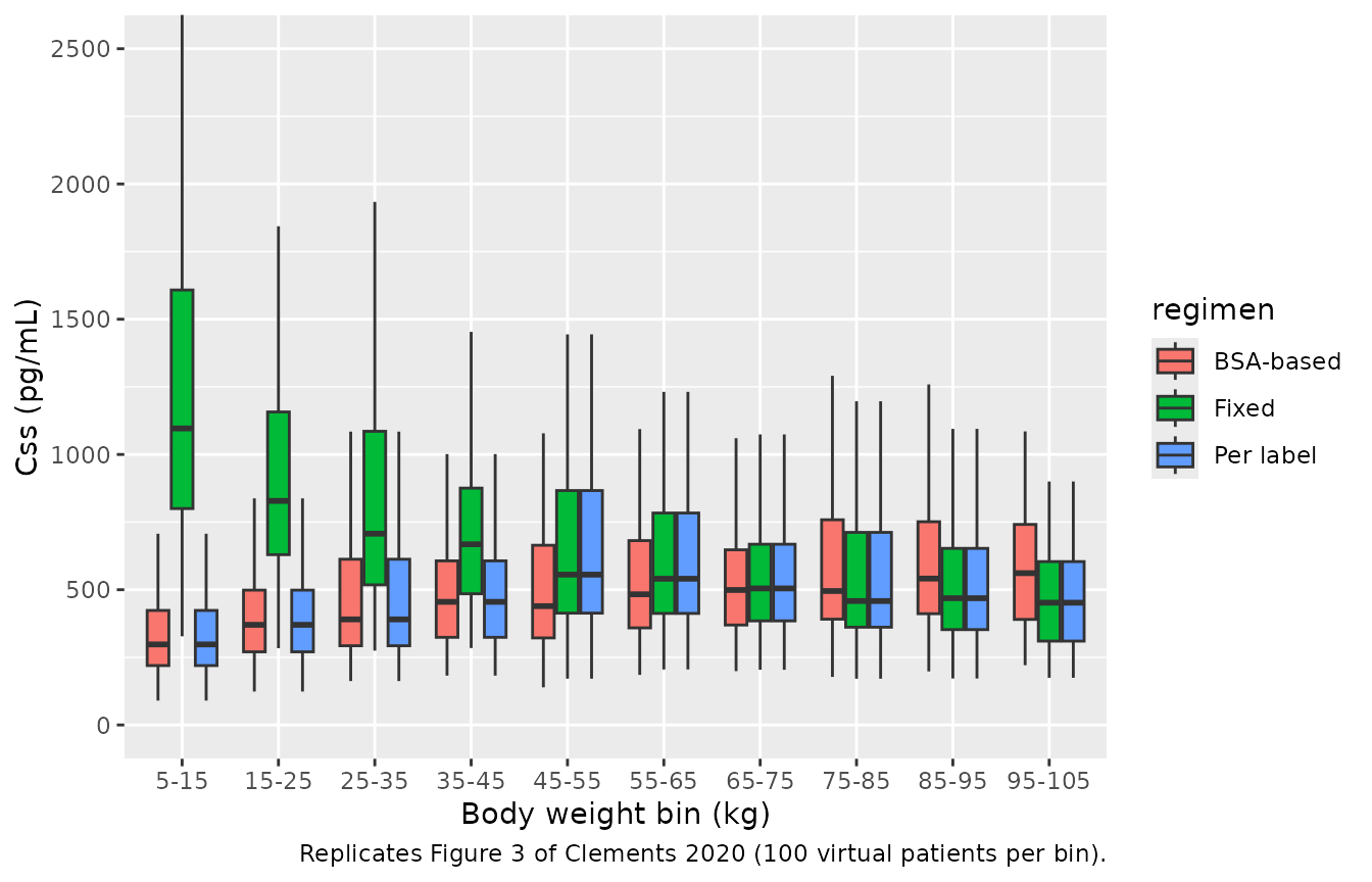
fig3_med <- fig3 |>
  dplyr::group_by(regimen, bin) |>
  dplyr::summarise(median_css = median(Css), .groups = "drop")
fig3_range <- fig3_med |>
  dplyr::group_by(regimen) |>
  dplyr::summarise(sim_min = min(median_css), sim_max = max(median_css)) |>
  dplyr::left_join(
    data.frame(
      regimen = c("Fixed", "BSA-based", "Per label"),
      paper_min = c(484, 391, 391), paper_max = c(873, 567, 603)
    ),
    by = "regimen"
  )
fig3_range |>
  dplyr::rename(
    "Regimen" = regimen,
    "Simulated min of bin medians" = sim_min,
    "Simulated max of bin medians" = sim_max,
    "Paper min" = paper_min,
    "Paper max" = paper_max
  ) |>
knitr::kable(digits = 0, caption = "Range of the per-bin median Css (Results 3.5).")| Regimen | Simulated min of bin medians | Simulated max of bin medians | Paper min | Paper max |
|---|---|---|---|---|
| BSA-based | 298 | 561 | 391 | 567 |
| Fixed | 452 | 1096 | 484 | 873 |
| Per label | 298 | 556 | 391 | 603 |
The adult-weight end of each range (the fixed-dose minimum, the BSA-based maximum, and the per-label maximum at the 45-55 kg bin) is reproduced closely. The paper’s lowest-bin medians are higher for BSA-based dosing and lower for fixed dosing than simulated here. The ratio of BSA-based to fixed Css for the same patient is exactly 15 x BSA / 28, independent of the model parameters, so the paper’s lowest-bin pair (391 / 873) implies a median BSA of about 0.84 m2 in its 5-15 kg bin, which is a 20-25 kg child. That points to the paper’s weight/BSA multivariate distribution (not published) rather than to the model parameters; the Livingston-Scott BSA at 10 kg is about 0.52 m2.
adult_end <- fig3_med |> dplyr::filter(bin %in% c("45-55", "95-105"))
fixed_top <- adult_end$median_css[adult_end$regimen == "Fixed" & adult_end$bin == "95-105"]
bsa_top <- adult_end$median_css[adult_end$regimen == "BSA-based" & adult_end$bin == "95-105"]
label_45 <- adult_end$median_css[adult_end$regimen == "Per label" & adult_end$bin == "45-55"]
stopifnot(
  abs(fixed_top / 484 - 1) < 0.15,
  abs(bsa_top / 567 - 1) < 0.15,
  abs(label_45 / 603 - 1) < 0.15
)
Assumptions and deviations
- Variance scale. Table 3 gives %CV only. The ESM states that IIV and residual variability were ‘expressed approximately as the percent coefficient of variation’, i.e. the approximation %CV/100 = SD of the log-scale random effect. The variances are therefore (CV/100)^2 (0.476^2 for CL, 0.643^2 for the residual-error eta) and the log-scale residual SD is 0.559.
-
IIV on the residual error. Encoded as the
per-subject log-scale residual SD
expSd * exp(etaexpSd), the usual NONMEM construction for ‘additive error in the log-domain with IIV’. The control stream is not published. - BSA formula. The paper does not state how BSA was calculated. The virtual cohorts use the weight-only Livingston-Scott formula because no heights are reported; this affects only the vignette cohorts, not the model.
- Virtual weights. The paper’s weight/BSA multivariate distribution for Figure 3 is not published; weights here are uniform within each 10-kg bin.
- Cohort size. 100 subjects per arm (Table 2 cohort) and per weight bin (Figure 3) instead of the paper’s 1000 per bin.
- Observation count. The abstract says 2417 concentrations; Results 3.1 gives 3629 after exclusions. The population metadata uses 3629.
- Screened covariates. Age, creatinine clearance, sex, AST, ALT, total bilirubin, albumin, LDH, hemoglobin, dose level and treatment cycle were screened graphically against the CL empirical Bayes estimates and not retained; none is in the model.
- Errata. No erratum was found for this article (checked 2026-09-25).