Isavuconazole (Cojutti 2021)
Source:vignettes/articles/Cojutti_2021_isavuconazole.Rmd
Cojutti_2021_isavuconazole.RmdModel and source
- Citation: Cojutti PG, Carnelutti A, Lazzarotto D, Sozio E, Candoni A, Fanin R, Tascini C, Pea F. Population Pharmacokinetics and Pharmacodynamic Target Attainment of Isavuconazole against Aspergillus fumigatus and Aspergillus flavus in Adult Patients with Invasive Fungal Diseases: Should Therapeutic Drug Monitoring for Isavuconazole Be Considered as Mandatory as for the Other Mold-Active Azoles? Pharmaceutics. 2021;13(12):2099. doi:10.3390/pharmaceutics13122099. PMCID PMC8708495.
- Description: Two-compartment population PK model for isavuconazole (dosed as the prodrug isavuconazonium sulfate, doses expressed as isavuconazole) in hospitalized adults treated for invasive fungal disease, mostly invasive pulmonary aspergillosis, with first-order oral absorption, oral bioavailability, 1-h intravenous infusion into the central compartment, and linear elimination (Cojutti 2021). No covariates were retained. Fitted non-parametrically with the NPAG algorithm in Pmetrics; the Table 3 medians are encoded as lognormal medians and the tabulated CV percentages as independent lognormal marginal variances.
- Article: https://doi.org/10.3390/pharmaceutics13122099 (PMC8708495; open access, CC BY)
Isavuconazole is a second-generation triazole approved for invasive aspergillosis and, in Europe, invasive mucormycosis. Cojutti and colleagues fitted a population PK model to routine therapeutic drug monitoring (TDM) data from 50 hospitalized adults at Udine, Italy, using the non-parametric adaptive grid (NPAG) algorithm in Pmetrics. They then ran Monte Carlo simulations of a 200 mg every 8 h loading dose for two days followed by 100, 200 or 300 mg once daily. The simulations report the probability that the trough falls below 1 mg/L or above the 5.13 mg/L toxicity threshold, and the probability of attaining AUC24h/MIC > 33.4 against Aspergillus fumigatus and A. flavus. The final model is a two-compartment model with first-order oral absorption, oral bioavailability and linear elimination. It has no covariates.
No erratum or correction was found on the journal landing page or in Europe PMC (checked 2026-09-30).
Population
knitr::kable(
  data.frame(
    Characteristic = c(
      "Patients", "Age (years)", "Male / female", "Body weight (kg)",
      "Albumin (g/L)", "Total bilirubin (mg/dL)", "Invasive pulmonary aspergillosis",
      "Oncohaematological malignancy", "Oral administration",
      "Troughs / peaks", "Observed Ctrough (mg/L)", "Observed Cpeak (mg/L)",
      "Treatment duration (days)"
    ),
    Value = c(
      "50", "61.5 (IQR 51.3-72.0)", "31 / 19", "65.0 (IQR 55.5-71.5)",
      "35.0 (IQR 28.4-40.0)", "0.28 (IQR 0.2-0.4)", "40 (80%)", "25 (50%)",
      "38 (76%)", "175 / 24", "3.68 (IQR 2.07-5.38)", "4.67 (IQR 3.78-5.96)",
      "48 (IQR 19-91)"
    )
  ),
  caption = "Cojutti 2021 Table 1 and Results."
)| Characteristic | Value |
|---|---|
| Patients | 50 |
| Age (years) | 61.5 (IQR 51.3-72.0) |
| Male / female | 31 / 19 |
| Body weight (kg) | 65.0 (IQR 55.5-71.5) |
| Albumin (g/L) | 35.0 (IQR 28.4-40.0) |
| Total bilirubin (mg/dL) | 0.28 (IQR 0.2-0.4) |
| Invasive pulmonary aspergillosis | 40 (80%) |
| Oncohaematological malignancy | 25 (50%) |
| Oral administration | 38 (76%) |
| Troughs / peaks | 175 / 24 |
| Observed Ctrough (mg/L) | 3.68 (IQR 2.07-5.38) |
| Observed Cpeak (mg/L) | 4.67 (IQR 3.78-5.96) |
| Treatment duration (days) | 48 (IQR 19-91) |
All patients received the labelled regimen of 200 mg every 8 h for 48 h followed by 200 mg once daily, orally or as a 1-h intravenous infusion. Troughs were drawn about 5 min before the daily dose, from at least 72 h after the start of therapy. Peaks were drawn 2 h after an oral dose or 0.5 h after the end of an infusion. No patient received a strong CYP3A4 inhibitor or inducer. Ten received mild or moderate CYP3A4 inhibitors. Race and ethnicity are not reported.
Source trace
knitr::kable(
  data.frame(
    Item = c(
      "lka", "lcl", "lvc", "lq", "lvp", "lfdepot",
      "etalka / etalcl / etalvc / etalq / etalvp",
      "IIV on Fos (not encoded)",
      "addSd", "propSd", "combined1()",
      "Two-compartment ODE, first-order oral input",
      "1-h intravenous infusion into central",
      "Cc = central / vc",
      "AGE, CONMED_CYP3A4_INH (excluded)",
      "WT, SEXF, ALB, TBILI, ALT, AST, GGT (excluded)"
    ),
    Value = c(
      "log(22.64) 1/h", "log(1.33) L/h", "log(102.58) L", "log(5.08) L/h",
      "log(385.93) L", "log(1.00)",
      "0.02423 / 0.3436 / 0.2023 / 0.7867 / 0.5558",
      "CV 7.42%",
      "0.012 mg/L", "0.378", "linear sum of SDs",
      "depot -> central <-> peripheral1",
      "dosing only", "mg / L = mg/L",
      "tested on CL, not retained",
      "Ctrough regression only"
    ),
    Source = c(
      rep("Table 3, Median row", 6),
      "Table 3, CV (%) row, omega^2 = log(CV^2 + 1)",
      "Table 3, CV (%) row; see Assumptions",
      "Methods 2.2: C0 = 0.006 x G = 2",
      "Methods 2.2: C1 = 0.189 x G = 2",
      "Methods 2.2: SD = C0 + C1 x C (Pmetrics polynomial)",
      "Methods 2.2; Results 3.2",
      "Methods 2.1 ('0.5 h after a 1 h intravenous infusion')",
      "Units declaration",
      "Results 3.2",
      "Table 2 (mixed-effect regression on Ctrough)"
    )
  )
)| Item | Value | Source |
|---|---|---|
| lka | log(22.64) 1/h | Table 3, Median row |
| lcl | log(1.33) L/h | Table 3, Median row |
| lvc | log(102.58) L | Table 3, Median row |
| lq | log(5.08) L/h | Table 3, Median row |
| lvp | log(385.93) L | Table 3, Median row |
| lfdepot | log(1.00) | Table 3, Median row |
| etalka / etalcl / etalvc / etalq / etalvp | 0.02423 / 0.3436 / 0.2023 / 0.7867 / 0.5558 | Table 3, CV (%) row, omega^2 = log(CV^2 + 1) |
| IIV on Fos (not encoded) | CV 7.42% | Table 3, CV (%) row; see Assumptions |
| addSd | 0.012 mg/L | Methods 2.2: C0 = 0.006 x G = 2 |
| propSd | 0.378 | Methods 2.2: C1 = 0.189 x G = 2 |
| combined1() | linear sum of SDs | Methods 2.2: SD = C0 + C1 x C (Pmetrics polynomial) |
| Two-compartment ODE, first-order oral input | depot -> central <-> peripheral1 | Methods 2.2; Results 3.2 |
| 1-h intravenous infusion into central | dosing only | Methods 2.1 (‘0.5 h after a 1 h intravenous infusion’) |
| Cc = central / vc | mg / L = mg/L | Units declaration |
| AGE, CONMED_CYP3A4_INH (excluded) | tested on CL, not retained | Results 3.2 |
| WT, SEXF, ALB, TBILI, ALT, AST, GGT (excluded) | Ctrough regression only | Table 2 (mixed-effect regression on Ctrough) |
Choice of typical values
Table 3 prints the mean, SD, CV and median of each parameter’s NPAG distribution, and the two columns differ a lot for the two distribution parameters. For Q the mean is 16.78 L/h and the median 5.08 L/h. For Vp the mean is 735 L and the median 386 L. The text uses both columns. The Discussion quotes the mean CL (1.52 L/h) as “the median CL estimate”. It also quotes “the wide median volume of distribution (488.51 L)”, which is the sum of the two medians (102.58 + 385.93) and not of the two means (824.74 L).
The paper’s own Monte Carlo output decides which column to use. Below, the Table 4 simulation is re-run with each column. The CV is the same in both runs, because Table 3’s CV is SD / mean for every row. The residual error is left out, because the paper’s Table 4 describes true troughs. The oral route is used, because Methods does not give the simulation route and F is 1 at the median.
md_levels <- c(100, 200, 300)
days <- c(2, 7, 14, 21, 28, 60)
# AUC24 needs a within-day grid; the trough is the value at the day's end
# (24 * day h), which is also the time of the next oral dose. An oral dose
# enters the depot, so Cc at that instant is still the pre-dose trough.
grid <- sort(unique(c(0, unlist(lapply(days, function(d) {
  24 * (d - 1) + c(0, 0.25, 0.5, 1, 1.5, 2, 3, 4, 6, 8, 12, 16, 20, 24)
})))))

make_events <- function(md) {
  rxode2::et(amt = 200, ii = 8, addl = 5, cmt = "depot") |>
    rxode2::et(time = 48, amt = md, ii = 24, addl = 60, cmt = "depot") |>
    rxode2::et(grid, cmt = "central")
}

n_per_arm <- 200
simulate_arms <- function(model, label) {
  bind_rows(lapply(md_levels, function(md) {
    s <- rxode2::rxSolve(model, make_events(md), nSub = n_per_arm,
                         returnType = "data.frame")
    # A single event table replicated with nSub returns the subject index as
    # sim.id rather than id.
    if (!"id" %in% names(s)) s$id <- s$sim.id
    s$md <- md
    s$column <- label
    s
  }))
}

# The mean column. Fos mean 0.95; no IIV on Fos in either run.
mod_mean <- mod |>
  ini(lka = log(22.64), lcl = log(1.52), lvc = log(89.50), lq = log(16.78),
      lvp = log(735.24), lfdepot = log(0.95))
#> ℹ parameter labels from comments will be replaced by 'label()'
#> ℹ change initial estimate of `lka` to `3.11971825333498`
#> ℹ change initial estimate of `lcl` to `0.418710334858185`
#> ℹ change initial estimate of `lvc` to `4.49423862528081`
#> ℹ change initial estimate of `lq` to `2.82018770103906`
#> ℹ change initial estimate of `lvp` to `6.60019697652556`
#> ℹ change initial estimate of `lfdepot` to `-0.0512932943875506`

rxode2::rxSetSeed(20211206)
sim_med <- simulate_arms(mod, "Median (encoded)")
#> ℹ parameter labels from comments will be replaced by 'label()'
rxode2::rxSetSeed(20211206)
sim_mean <- simulate_arms(mod_mean, "Mean")
sim_all <- bind_rows(sim_med, sim_mean)
troughs <- sim_all |>
  filter(time %in% (24 * days)) |>
  mutate(day = time / 24)

sim_t4 <- troughs |>
  group_by(column, md, day) |>
  summarise(
    lt1 = 100 * mean(Cc < 1),
    mid = 100 * mean(Cc >= 1 & Cc <= 5.13),
    gt5 = 100 * mean(Cc > 5.13),
    .groups = "drop"
  )

# Cojutti 2021 Table 4. The Day 2 (end of loading) column is common to all
# three maintenance doses.
pub_t4 <- tibble::tribble(
  ~md, ~day, ~lt1_pub, ~mid_pub, ~gt5_pub,
  100, 2, 1.7, 85.2, 13.1,
  100, 7, 21.7, 76.4, 1.9,
  100, 14, 16.4, 81.5, 2.1,
  100, 21, 12.9, 84.6, 2.5,
  100, 28, 12.0, 83.8, 4.2,
  100, 60, 11.7, 81.1, 7.2,
  200, 2, 1.7, 85.2, 13.1,
  200, 7, 4.1, 84.3, 11.6,
  200, 14, 1.8, 80.4, 17.8,
  200, 21, 1.3, 73.6, 25.1,
  200, 28, 1.0, 71.3, 27.7,
  200, 60, 1.1, 59.7, 39.2,
  300, 2, 1.7, 85.2, 13.1,
  300, 7, 0.8, 76.9, 22.3,
  300, 14, 0.2, 60.6, 39.2,
  300, 21, 0.2, 48.6, 51.2,
  300, 28, 0.1, 46.9, 53.0,
  300, 60, 0.1, 26.6, 73.2
)

t4 <- sim_t4 |>
  left_join(pub_t4, by = c("md", "day")) |>
  mutate(abs_diff = (abs(lt1 - lt1_pub) + abs(mid - mid_pub) + abs(gt5 - gt5_pub)) / 3)

knitr::kable(
  t4 |>
    filter(column == "Median (encoded)") |>
    transmute(md, day,
              lt1 = sprintf("%.1f (%.1f)", lt1, lt1_pub),
              mid = sprintf("%.1f (%.1f)", mid, mid_pub),
              gt5 = sprintf("%.1f (%.1f)", gt5, gt5_pub)) |>
    dplyr::rename("MD (mg/day)" = md, "Day" = day,
                  "Ctrough < 1 mg/L, % (published)" = lt1,
                  "1-5.13 mg/L, % (published)" = mid,
                  "> 5.13 mg/L, % (published)" = gt5),
  caption = paste("Replicates Table 4 of Cojutti 2021 with the encoded (median)",
                  "parameters; published values in parentheses.")
)| MD (mg/day) | Day | Ctrough < 1 mg/L, % (published) | 1-5.13 mg/L, % (published) | > 5.13 mg/L, % (published) |
|---|---|---|---|---|
| 100 | 2 | 0.5 (1.7) | 80.0 (85.2) | 19.5 (13.1) |
| 100 | 7 | 14.0 (21.7) | 84.5 (76.4) | 1.5 (1.9) |
| 100 | 14 | 12.5 (16.4) | 83.5 (81.5) | 4.0 (2.1) |
| 100 | 21 | 12.0 (12.9) | 83.0 (84.6) | 5.0 (2.5) |
| 100 | 28 | 12.0 (12.0) | 82.0 (83.8) | 6.0 (4.2) |
| 100 | 60 | 8.5 (11.7) | 81.0 (81.1) | 10.5 (7.2) |
| 200 | 2 | 0.0 (1.7) | 76.0 (85.2) | 24.0 (13.1) |
| 200 | 7 | 3.5 (4.1) | 82.5 (84.3) | 14.0 (11.6) |
| 200 | 14 | 1.5 (1.8) | 76.0 (80.4) | 22.5 (17.8) |
| 200 | 21 | 1.0 (1.3) | 66.0 (73.6) | 33.0 (25.1) |
| 200 | 28 | 1.0 (1.0) | 59.5 (71.3) | 39.5 (27.7) |
| 200 | 60 | 1.0 (1.1) | 44.5 (59.7) | 54.5 (39.2) |
| 300 | 2 | 1.5 (1.7) | 78.5 (85.2) | 20.0 (13.1) |
| 300 | 7 | 0.5 (0.8) | 81.0 (76.9) | 18.5 (22.3) |
| 300 | 14 | 0.5 (0.2) | 51.0 (60.6) | 48.5 (39.2) |
| 300 | 21 | 0.5 (0.2) | 42.5 (48.6) | 57.0 (51.2) |
| 300 | 28 | 0.5 (0.1) | 36.5 (46.9) | 63.0 (53.0) |
| 300 | 60 | 0.5 (0.1) | 23.5 (26.6) | 76.0 (73.2) |
fit_summary <- t4 |>
  group_by(column) |>
  summarise(
    mean_abs_diff = mean(abs_diff),
    lt1_end_of_loading = mean(lt1[day == 2]),
    .groups = "drop"
  )
knitr::kable(
  fit_summary |>
    dplyr::rename("Table 3 column" = column,
                  "Mean |difference| from Table 4 (points)" = mean_abs_diff,
                  "Ctrough < 1 mg/L at end of loading, % (published 1.7)" = lt1_end_of_loading),
  digits = 1,
  caption = "Agreement of each Table 3 column with the published Monte Carlo output."
)| Table 3 column | Mean |difference| from Table 4 (points) | Ctrough < 1 mg/L at end of loading, % (published 1.7) |
|---|---|---|
| Mean | 7.8 | 17.3 |
| Median (encoded) | 4.4 | 0.7 |
The median column reproduces Table 4 closely. Both the fraction of troughs below 1 mg/L at the end of loading and the build-up of troughs above 5.13 mg/L over two months come out close to the published values. The mean column puts many more troughs below 1 mg/L at the end of loading, because its larger Vp and Q move more drug into the peripheral compartment during loading. So the medians are encoded.
fs <- setNames(fit_summary$mean_abs_diff, fit_summary$column)
lt <- setNames(fit_summary$lt1_end_of_loading, fit_summary$column)
stopifnot(
  # Centre of agreement over all 18 cells. Realised 3.0-5.1 over seven seeds
  # and at 1 and 4 threads (the mean column gives 7.8-9.9), so 7 leaves room
  # for the draw.
  fs[["Median (encoded)"]] < 7,
  # End of loading, Ctrough < 1 mg/L: realised 0.2-1.5 percent with the
  # median column and 17-20 percent with the mean column over the same runs.
  # The 8 percent split sits well clear of both.
  lt[["Median (encoded)"]] < 8,
  lt[["Mean"]] > 8
)
Replicate Figure 4
fig4 <- troughs |>
  filter(column == "Median (encoded)") |>
  group_by(md, day) |>
  summarise(
    q05 = quantile(Cc, 0.05), q25 = quantile(Cc, 0.25), q50 = median(Cc),
    q75 = quantile(Cc, 0.75), q95 = quantile(Cc, 0.95), .groups = "drop"
  ) |>
  mutate(day = factor(day), md = paste("MD", md, "mg daily"))

ggplot(fig4, aes(x = day)) +
  geom_boxplot(aes(ymin = q05, lower = q25, middle = q50, upper = q75, ymax = q95),
               stat = "identity", fill = "grey85") +
  geom_hline(yintercept = 5.13, linetype = "dashed") +
  facet_wrap(~md) +
  labs(x = "Day of treatment", y = "Isavuconazole Ctrough (mg/L)") +
  theme_bw()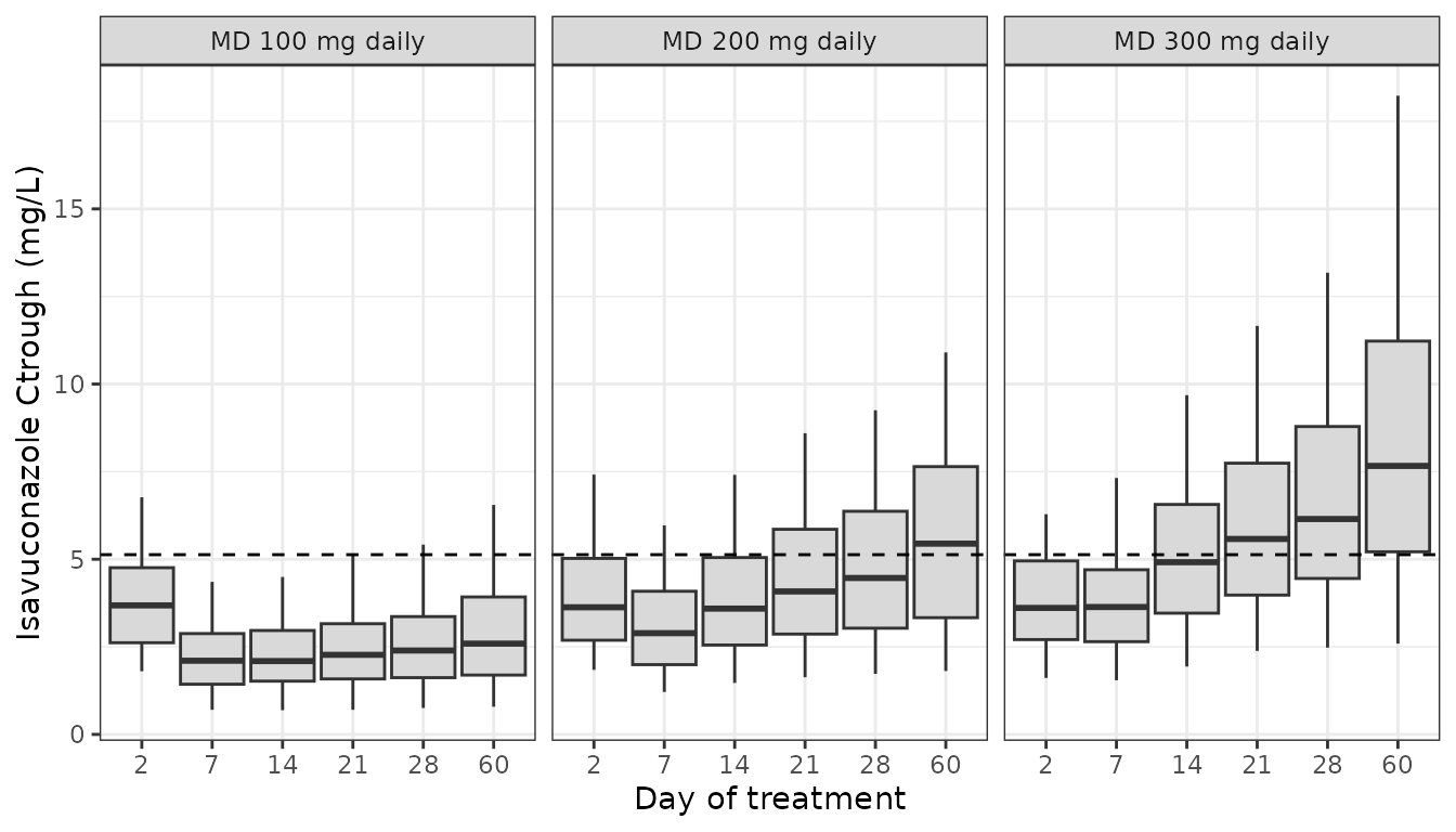
Replicates Figure 4 of Cojutti 2021: boxes are the median and 25th-75th percentiles, whiskers the 5th-95th percentiles, and the dashed line is the 5.13 mg/L toxicity threshold. Troughs build up over the whole two months, as the paper reports. The typical terminal half-life of this parameter set is about 300 h, so steady state is reached only after several weeks.
Probability of target attainment
Figure 5 reports that the standard 200 mg maintenance dose “achieved optimal PTAs” (at least 90%) at the 1 mg/L EUCAST breakpoint on Day 7, for a target of AUC24h/MIC > 33.4. The Table 5 cumulative fractions of response need the EUCAST MIC distributions, which the paper does not tabulate, so they are not recomputed here.
nca_in <- sim_med |>
  filter(!is.na(Cc)) |>
  mutate(treatment = paste("MD", md, "mg"), id = paste(md, id)) |>
  select(id, time, Cc, treatment)

# Dose records per subject: LD at 0, 8, ..., 40 h, then MD every 24 h from 48 h.
dose_times <- c(seq(0, 40, by = 8), seq(48, 48 + 24 * 60, by = 24))
doses <- nca_in |>
  distinct(id, treatment) |>
  tidyr::crossing(time = dose_times) |>
  mutate(amt = ifelse(time < 48, 200, as.numeric(sub("MD ([0-9]+) mg", "\\1", treatment))))

conc_obj <- PKNCA::PKNCAconc(nca_in, Cc ~ time | treatment + id)
dose_obj <- PKNCA::PKNCAdose(doses, amt ~ time | treatment + id)
intervals <- data.frame(
  start = 24 * (days - 1), end = 24 * days,
  auclast = TRUE, cmax = TRUE, cmin = TRUE
)
nca_res <- PKNCA::pk.nca(PKNCA::PKNCAdata(conc_obj, dose_obj, intervals = intervals))

nca_tab <- as.data.frame(nca_res$result) |>
  filter(PPTESTCD %in% c("auclast", "cmax", "cmin")) |>
  mutate(day = end / 24)

pta <- nca_tab |>
  filter(PPTESTCD == "auclast") |>
  group_by(treatment, day) |>
  summarise(
    median_auc24 = median(PPORRES),
    pta_mic1 = 100 * mean(PPORRES / 1 > 33.4),
    .groups = "drop"
  )
knitr::kable(
  pta |>
    dplyr::rename("Regimen" = treatment, "Day" = day,
                  "Median AUC24 (mg*h/L)" = median_auc24,
                  "PTA at MIC 1 mg/L (%)" = pta_mic1),
  digits = 1,
  caption = "Simulated AUC24 and PTA of AUC24/MIC > 33.4 at MIC = 1 mg/L."
)| Regimen | Day | Median AUC24 (mg*h/L) | PTA at MIC 1 mg/L (%) |
|---|---|---|---|
| MD 100 mg | 2 | 87.4 | 99.5 |
| MD 100 mg | 7 | 58.6 | 86.5 |
| MD 100 mg | 14 | 61.3 | 87.5 |
| MD 100 mg | 21 | 63.6 | 87.5 |
| MD 100 mg | 28 | 65.8 | 87.0 |
| MD 100 mg | 60 | 69.0 | 89.0 |
| MD 200 mg | 2 | 84.9 | 100.0 |
| MD 200 mg | 7 | 83.6 | 99.0 |
| MD 200 mg | 14 | 99.9 | 100.0 |
| MD 200 mg | 21 | 112.4 | 100.0 |
| MD 200 mg | 28 | 122.8 | 100.0 |
| MD 200 mg | 60 | 148.7 | 100.0 |
| MD 300 mg | 2 | 84.3 | 98.5 |
| MD 300 mg | 7 | 111.1 | 99.5 |
| MD 300 mg | 14 | 140.8 | 99.5 |
| MD 300 mg | 21 | 161.7 | 99.5 |
| MD 300 mg | 28 | 175.5 | 99.5 |
| MD 300 mg | 60 | 210.8 | 99.5 |
pta200 <- pta$pta_mic1[pta$treatment == "MD 200 mg" & pta$day == 7]
# Figure 5: at least 90 percent at MIC 1 mg/L with 200 mg on Day 7. Allow
# 3-4 Monte Carlo SE at n = 200 below the claim.
stopifnot(pta200 > 85)
The simulated PTA at 1 mg/L on Day 7 with 200 mg daily is 99.0%, in line with the paper’s statement that the standard dose reaches at least 90% at the breakpoint.
Comparison with observed TDM values
The paper reports no NCA of its own. The nearest thing is the Table 1 summary of observed TDM concentrations under 200 mg daily, which pools troughs and peaks drawn at different times from Day 3 to several months. The table below compares these with the simulated Day 14 dosing interval under 200 mg daily. For an oral dose absorbed with a half-life of about 2 minutes, the 2-h post-dose peak is close to Cmax. This is a descriptive check and is not used as a gate.
published_tdm <- data.frame(
  treatment = "MD 200 mg",
  cmin = 3.68,
  cmax = 4.67
)
sim_day14 <- nca_res
sim_day14$result <- sim_day14$result |>
  filter(end == 24 * 14, PPTESTCD %in% c("cmin", "cmax"))

knitr::kable(
  nlmixr2lib::ncaComparisonTable(
    simulated = sim_day14,
    reference = published_tdm,
    by = "treatment",
    units = c(cmin = "mg/L", cmax = "mg/L"),
    tolerance_pct = 20
  ),
  caption = paste("Simulated Day 14 cmin / cmax (200 mg daily) against the observed",
                  "Table 1 TDM medians. * differs by >20%.")
)| NCA parameter | treatment | Reference | Simulated | % diff |
|---|---|---|---|---|
| Cmax (mg/L) | MD 200 mg | 4.67 | 5.42 | +16.1% |
| Cmin (mg/L) | MD 200 mg | 3.68 | 3.49 | -5.2% |
Steady-state closed-form check
For a linear model the steady-state AUC over a dosing interval equals F x Dose / CL. The typical patient is run for 150 days of 200 mg daily, which is more than 10 terminal half-lives, and PKNCA is applied to the last interval.
ev_ss <- rxode2::et(amt = 200, ii = 24, addl = 149, cmt = "depot") |>
  rxode2::et(c(0, 24 * 149 + c(0, 0.25, 0.5, 1, 2, 4, 8, 12, 16, 20, 24)), cmt = "central")
ss <- rxode2::rxSolve(rxode2::zeroRe(mod), ev_ss, returnType = "data.frame") |>
  filter(!is.na(Cc)) |>
  mutate(id = 1, treatment = "200 mg daily, typical")
#> ℹ parameter labels from comments will be replaced by 'label()'
#> ℹ omega/sigma items treated as zero: 'etalka', 'etalcl', 'etalvc', 'etalq', 'etalvp'
ss_dose <- data.frame(id = 1, treatment = "200 mg daily, typical",
                      time = seq(0, 24 * 149, by = 24), amt = 200)
ss_nca <- PKNCA::pk.nca(PKNCA::PKNCAdata(
  PKNCA::PKNCAconc(ss, Cc ~ time | treatment + id),
  PKNCA::PKNCAdose(ss_dose, amt ~ time | treatment + id),
  intervals = data.frame(start = 24 * 149, end = 24 * 150, auclast = TRUE)
))
auc_ss <- as.data.frame(ss_nca$result)$PPORRES[1]
auc_closed <- 1.00 * 200 / 1.33
c(PKNCA = auc_ss, closed_form = auc_closed)
#>       PKNCA closed_form
#>    150.2819    150.3759
# Deterministic; the only difference is trapezoidal error on the fast
# absorption peak and the few percent of steady state not yet reached.
stopifnot(abs(auc_ss / auc_closed - 1) < 0.05)
Assumptions and deviations
- Median column encoded. Table 3 gives both a mean and a median for each parameter. The medians are encoded because they reproduce the paper’s own Table 4 Monte Carlo output and the means do not (see “Choice of typical values”). The Discussion’s “median CL (1.52 L/h)” is the Table 3 mean.
- Lognormal marginals for a non-parametric fit. NPAG estimates a discrete joint distribution. The CV column is carried as independent lognormal marginals with omega^2 = log(CV^2 + 1), because covariances are not reported. Any multimodality in the NPAG distribution cannot be recovered from Table 3. The simulated trough distribution builds up a little faster than Table 4 after Day 21 (for example, 200 mg Day 60 above 5.13 mg/L). This is the expected sign of lognormal tails on Q and Vp. It is not a transcription error.
- No IIV on bioavailability. Fos has median 1.00, mean 0.95 and CV 7.42%. With the median at the upper bound of 1, a lognormal marginal would give F > 1 to half of the patients, and a logit-normal marginal is undefined. Bioavailability is therefore fixed at its typical value of 1 for every simulated patient. The Table 3 column header says “Fos (%)”, but the values are fractions.
- Ka. Table 3 gives the same mean and median for Ka (22.64 1/h, an absorption half-life of about 2 minutes). The data were troughs and a few 2-h peaks, so they carry almost no information on absorption. The value is encoded as printed.
-
Residual error. Methods gives the assay polynomial
SD = 0.006 + 0.189 x C and a gamma of 2. Pmetrics multiplies the assay
SD by gamma, so the encoded residual is 0.012 mg/L + 37.8% with the two
parts summed linearly (
combined1()). The 0.189 slope is larger than the “< 10%” inter-assay CV that Methods quotes. The paper does not say whether C1 absorbs extra variability, and the value is encoded as printed. - Monte Carlo settings. Methods does not give the route or the error model of the Table 4 simulation. Here the simulation is oral with no residual error, and the trough is taken at the end of each named day (24 x day h). Troughs with added residual error fit Table 4 worse; for example, they put about 5% below 1 mg/L at the end of loading against the published 1.7%.
-
Covariates. The population model retained none. Age
and mild or moderate CYP3A4 inhibitors were tested on CL and did not
improve the fit. The other Table 2 variables come from a separate
mixed-effect regression on Ctrough and were never part of the PK model.
All of them are listed in
covariatesDataExcluded. - Dose units. Doses are isavuconazole equivalents (200 mg isavuconazole = 372 mg isavuconazonium sulfate), as in the paper.