Lamivudine (Moore 1999)
Source:vignettes/articles/Moore_1999_lamivudine.Rmd
Moore_1999_lamivudine.RmdModel and source
- Citation: Moore KHP, Yuen GJ, Hussey EK, Pakes GE, Eron JJ Jr, Bartlett JA. Population pharmacokinetics of lamivudine in adult human immunodeficiency virus-infected patients enrolled in two phase III clinical trials. Antimicrob Agents Chemother. 1999;43(12):3025-3029. doi:10.1128/aac.43.12.3025
- Description: One-compartment population PK model for oral lamivudine in HIV-1-infected adults pooled from the NUCA3001 and NUCA3002 phase III trials (Moore 1999); CL/F scales with a Cockcroft-Gault-style renal function index ((140 - AGE)/(CREAT * 100), * 0.85 if female) raised to an estimated power and with linear body weight, V/F and ka carry no covariates
- Article: https://doi.org/10.1128/aac.43.12.3025
Population
Moore 1999 pooled data from two large phase III lamivudine efficacy/safety trials, NUCA3001 (245 patients) and NUCA3002 (149 patients), giving 394 HIV-1-infected adults with adequate dosing and sample-time documentation and 1,477 evaluable serum lamivudine concentrations. The cohort was predominantly male (87%), mean age 35.7 years (range 19-64), mean weight 74.2 kg (range 37.2-138.5), 62% Caucasian / 15% Black / 22% Hispanic / 1% Other, and well-distributed across CDC classes A/B/C (62%/32%/6%). Mean calculated Cockcroft-Gault creatinine clearance was 97.4 mL/min; only three patients had CrCl < 60 mL/min, so the renal-impairment range was sparsely sampled. Dosing was oral lamivudine 150 mg BID or 300 mg BID, either alone or with zidovudine 200 mg TID. Demographics are summarised in Table 1 of the source.
The same information is available programmatically:
readModelDb("Moore_1999_lamivudine")$population after the
model is loaded.
Source trace
Per-parameter origin (also recorded as in-file comments next to each
ini() entry of
inst/modeldb/specificDrugs/Moore_1999_lamivudine.R):
| Equation / parameter | Value | Source location |
|---|---|---|
lka |
log(4.65) | Table 2 (theta_3 = 4.65 h^-1) |
lcl |
log(25.1) | Table 2 (theta_1 = 25.1 L/h, CL/F reference) |
lvc |
log(128) | Table 2 (theta_2 = 128 L, V/F) |
e_renal_cl |
0.468 | Table 2 (theta_4 = 0.468, renal-function exponent) |
etalcl |
0.124 | Table 2 (eta on CL/F = 0.124, %CV = 35.2) |
etalvc |
0.0965 | Table 2 (eta on V/F = 0.0965, %CV = 31.1) |
expSd |
0.404 | Table 2 (epsilon variance = 0.163, %CV = 40.4); footnote f: error model F * EXP(eps1) |
rfi formula |
n/a | Table 2 footnote d (male: (140 - age)/(SCR * 100); female: same * 0.85) |
d/dt(depot), d/dt(central)
|
n/a | Methods page 3026 (“one-compartment open model with first-order elimination (ADVAN2 TRANS2)”) |
Cc <- central / vc |
n/a | Standard linear-CL parameterisation; dose mg, volume L -> mg/L = ug/mL |
Cc ~ lnorm(expSd) |
n/a | Table 2 footnote f (F * EXP(eps1)) |
Virtual cohort
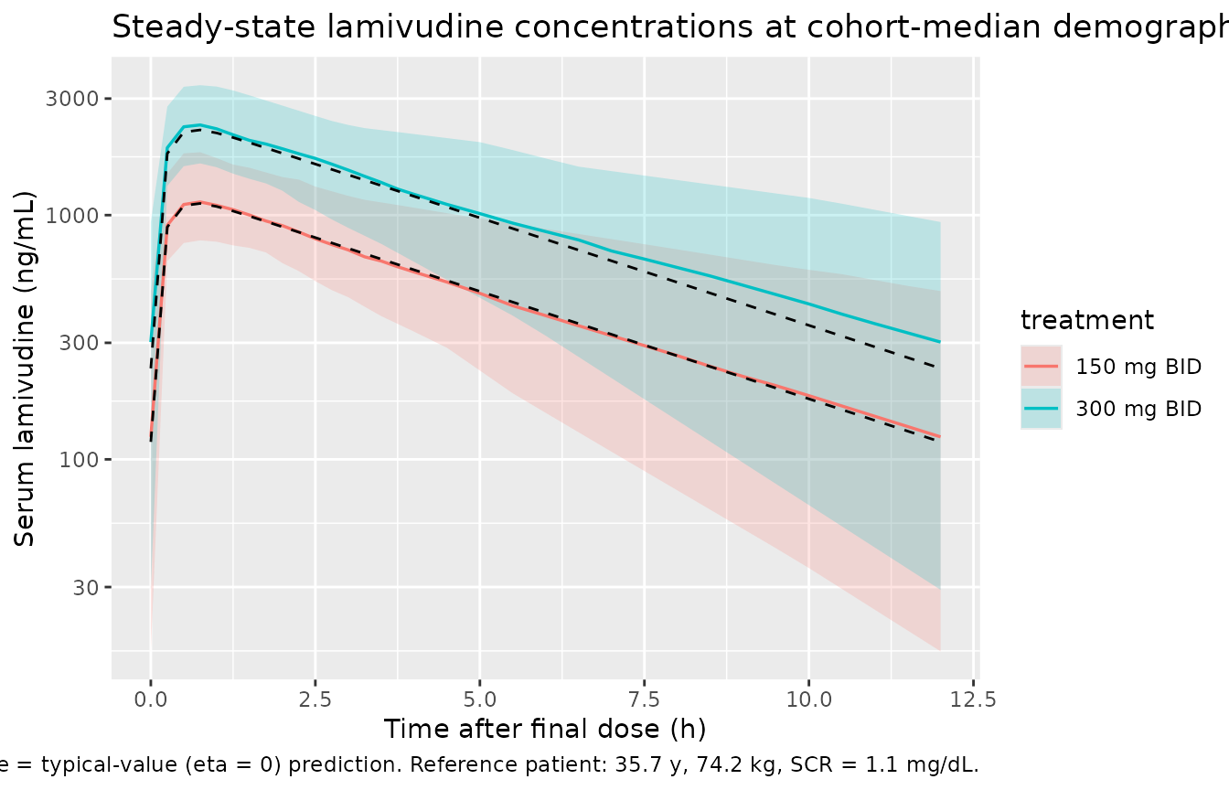
Original observed data are not publicly available. The cohort below is a virtual reproduction of the two licensed dosing regimens (150 mg BID and 300 mg BID) at the cohort-median demographics (35.7 years, 74.2 kg, serum creatinine 1.1 mg/dL, 87% male) sampled densely over a single dosing interval after multiple dosing has reached steady state.
set.seed(19991201L)

n_per_group  <- 100L
ref_age      <- 35.7   # years (Table 1 cohort mean)
ref_wt       <- 74.2   # kg (Table 1 cohort mean)
ref_creat    <- 1.1    # mg/dL (Table 1 cohort mean)
ref_sexf_pct <- 0.13   # 13% female per Table 1
tau          <- 12     # h, BID dosing
n_doses      <- 14     # ~7 days BID, well past SS for kel ~ 25/128 = 0.196/h, t1/2 ~3.5 h
sample_hours <- c(seq(0, 4, by = 0.25), seq(4.5, 12, by = 0.5))

make_cohort <- function(dose_amt_mg, id_offset) {
  ids <- seq_len(n_per_group) + id_offset
  # Per-subject random sex (matching cohort female %); other covariates fixed at mean
  sexf <- rbinom(n_per_group, size = 1, prob = ref_sexf_pct)
  cov_tbl <- tibble::tibble(
    id    = ids,
    WT    = ref_wt,
    AGE   = ref_age,
    CREAT = ref_creat,
    SEXF  = sexf,
    treatment = paste0(dose_amt_mg, " mg BID")
  )
  dose_times <- seq(0, by = tau, length.out = n_doses)
  dose_rows <- tidyr::expand_grid(id = ids, time = dose_times) |>
    dplyr::mutate(amt = dose_amt_mg, evid = 1L, cmt = 1L)
  ss_start <- max(dose_times)
  obs_times <- ss_start + sample_hours
  obs_rows <- tidyr::expand_grid(id = ids, time = obs_times) |>
    dplyr::mutate(amt = 0, evid = 0L, cmt = NA_integer_)
  dplyr::bind_rows(dose_rows, obs_rows) |>
    dplyr::left_join(cov_tbl, by = "id") |>
    dplyr::arrange(id, time, dplyr::desc(evid))
}

events <- dplyr::bind_rows(
  make_cohort(150,   0L),
  make_cohort(300, 200L)
)

stopifnot(!anyDuplicated(unique(events[, c("id", "time", "evid")])))
Simulation
mod <- rxode2::rxode2(readModelDb("Moore_1999_lamivudine"))
#> ℹ parameter labels from comments will be replaced by 'label()'

sim <- rxode2::rxSolve(
  mod,
  events = events,
  keep   = c("WT", "AGE", "CREAT", "SEXF", "treatment")
) |>
  as.data.frame()
Deterministic typical-value lines (zeroed-eta) for the published-parameter profile per treatment:
mod_typical <- mod |> rxode2::zeroRe()
sim_typical <- rxode2::rxSolve(
  mod_typical,
  events = events |> dplyr::filter(id %in% c(1L, 201L)),
  keep   = c("treatment")
) |>
  as.data.frame()
#> ℹ omega/sigma items treated as zero: 'etalcl', 'etalvc'
#> Warning: multi-subject simulation without without 'omega'
Steady-state concentration vs time
The published paper itself does not show a steady-state concentration-time plot, but Figure 1 illustrates the model fit (predicted vs observed) through serum concentrations spanning roughly 0-8000 ng/mL. The plot below reproduces the steady-state concentration profile under the two licensed dosing regimens at the cohort-median demographics.
ss_start <- max(events$time[events$evid == 1L])

sim_ss <- sim |>
  dplyr::filter(time >= ss_start, !is.na(Cc)) |>
  dplyr::mutate(time_post_dose = time - ss_start,
                Cc_ngml = Cc * 1000)  # convert mg/L -> ng/mL for paper units

sim_typical_ss <- sim_typical |>
  dplyr::filter(time >= ss_start, !is.na(Cc)) |>
  dplyr::mutate(time_post_dose = time - ss_start,
                Cc_ngml = Cc * 1000)

q_ss <- sim_ss |>
  dplyr::group_by(treatment, time_post_dose) |>
  dplyr::summarise(
    Q05 = stats::quantile(Cc_ngml, 0.05, na.rm = TRUE),
    Q50 = stats::quantile(Cc_ngml, 0.50, na.rm = TRUE),
    Q95 = stats::quantile(Cc_ngml, 0.95, na.rm = TRUE),
    .groups = "drop"
  )

ggplot(q_ss, aes(time_post_dose, Q50, fill = treatment, colour = treatment)) +
  geom_ribbon(aes(ymin = Q05, ymax = Q95), alpha = 0.2, colour = NA) +
  geom_line(linewidth = 0.6) +
  geom_line(
    data = sim_typical_ss,
    aes(time_post_dose, Cc_ngml, group = treatment),
    linewidth = 0.5, linetype = "dashed", colour = "black", inherit.aes = FALSE
  ) +
  scale_y_log10() +
  labs(
    x = "Time after final dose (h)",
    y = "Serum lamivudine (ng/mL)",
    title = "Steady-state lamivudine concentrations at cohort-median demographics",
    caption = "Median + 5-95% interval over 100 simulated subjects per regimen; dashed line = typical-value (eta = 0) prediction. Reference patient: 35.7 y, 74.2 kg, SCR = 1.1 mg/dL."
  )
Renal-function effect on typical CL/F
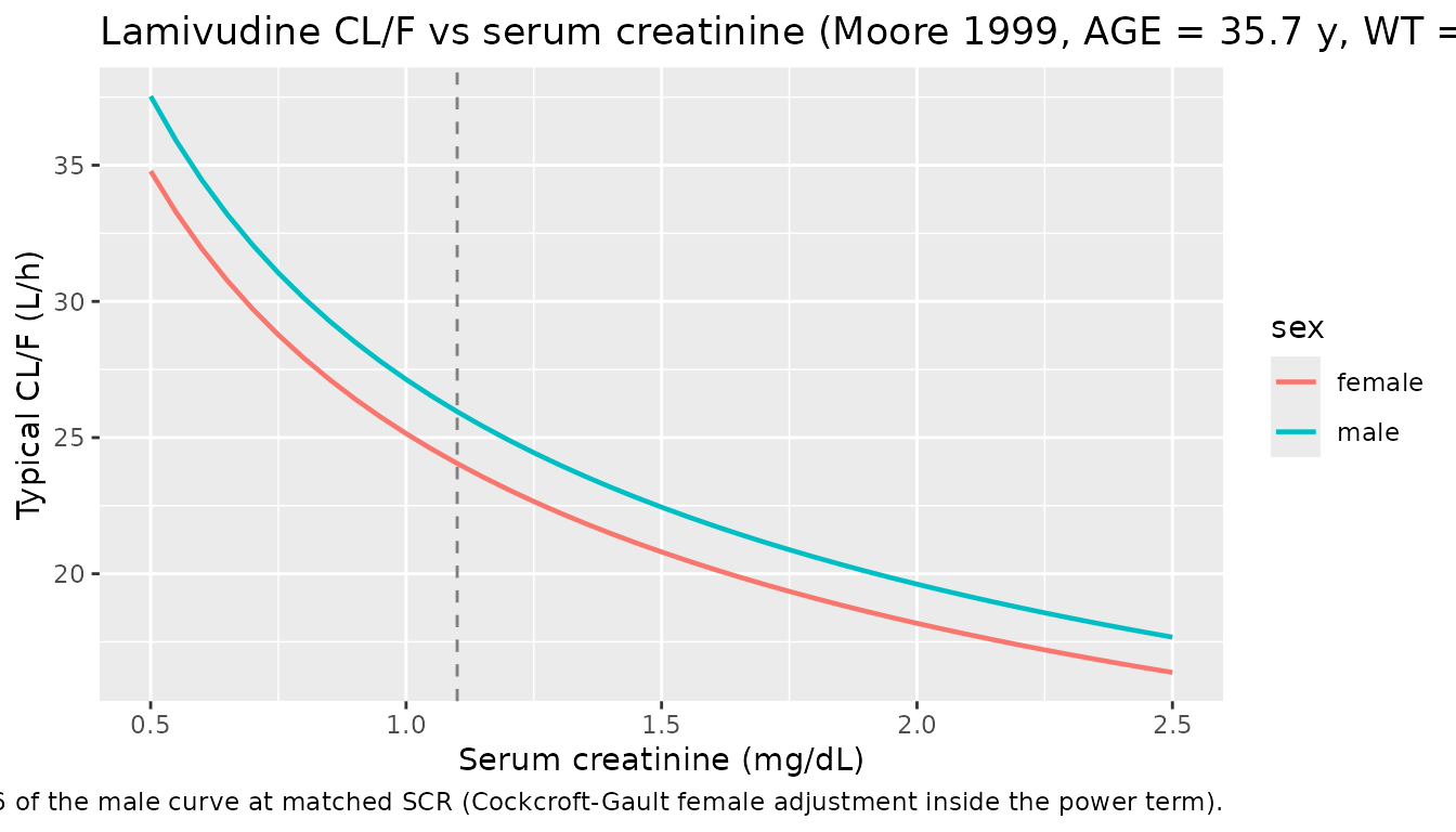
Table 2 footnote d encodes a Cockcroft-Gault-style renal-function index raised to the estimated exponent 0.468 on CL/F. The plot below traces typical CL/F across the patient’s serum creatinine at fixed age (35.7 y) and weight (74.2 kg), separately for male and female.
theta1     <- 25.1
e_renal    <- 0.468
creat_grid <- seq(0.5, 2.5, by = 0.05)

mk_cl <- function(sexf) {
  rfi <- (140 - ref_age) / (creat_grid * 100) * (1 - 0.15 * sexf)
  theta1 * rfi^e_renal * (ref_wt / 70)
}

cl_df <- dplyr::bind_rows(
  tibble::tibble(CREAT = creat_grid, CL = mk_cl(0L), sex = "male"),
  tibble::tibble(CREAT = creat_grid, CL = mk_cl(1L), sex = "female")
)

ggplot(cl_df, aes(CREAT, CL, colour = sex)) +
  geom_line(linewidth = 0.8) +
  geom_vline(xintercept = ref_creat, linetype = "dashed", colour = "grey50") +
  labs(
    x = "Serum creatinine (mg/dL)",
    y = "Typical CL/F (L/h)",
    title = "Lamivudine CL/F vs serum creatinine (Moore 1999, AGE = 35.7 y, WT = 74.2 kg)",
    caption = "Dashed grey line = cohort mean serum creatinine (1.1 mg/dL); the female curve is uniformly ~ 0.85^0.468 = 0.926 of the male curve at matched SCR (Cockcroft-Gault female adjustment inside the power term)."
  )
PKNCA validation (steady-state AUC0-tau, Cmax, Cmin)
ss_dose_df <- events |>
  dplyr::filter(evid == 1L, time == ss_start) |>
  dplyr::select(id, time, amt, treatment)

sim_ss_pknca <- sim_ss |>
  dplyr::select(id, time, Cc, treatment) |>
  dplyr::filter(!is.na(Cc))

conc_obj <- PKNCA::PKNCAconc(sim_ss_pknca, Cc ~ time | treatment + id,
                             concu = "mg/L", timeu = "h")
dose_obj <- PKNCA::PKNCAdose(ss_dose_df, amt ~ time | treatment + id,
                             doseu = "mg",
                             route = "extravascular")

intervals <- data.frame(
  start    = ss_start,
  end      = ss_start + tau,
  cmax     = TRUE,
  tmax     = TRUE,
  cmin     = TRUE,
  auclast  = TRUE,
  cav      = TRUE
)

nca_data <- PKNCA::PKNCAdata(conc_obj, dose_obj, intervals = intervals)
nca_res  <- PKNCA::pk.nca(nca_data)

nca_summary <- as.data.frame(nca_res$result) |>
  dplyr::filter(PPTESTCD %in% c("cmax", "tmax", "cmin", "auclast", "cav")) |>
  dplyr::group_by(treatment, PPTESTCD) |>
  dplyr::summarise(
    median = stats::median(PPORRES, na.rm = TRUE),
    p05    = stats::quantile(PPORRES, 0.05, na.rm = TRUE),
    p95    = stats::quantile(PPORRES, 0.95, na.rm = TRUE),
    .groups = "drop"
  )

knitr::kable(
  nca_summary,
  caption = "Simulated lamivudine steady-state NCA (mg/L for concentrations, mg*h/L for AUC, h for tmax)."
)| treatment | PPTESTCD | median | p05 | p95 |
|---|---|---|---|---|
| 150 mg BID | auclast | 5.7130621 | 3.4052883 | 11.0115164 |
| 150 mg BID | cav | 0.4760885 | 0.2837740 | 0.9176264 |
| 150 mg BID | cmax | 1.1321441 | 0.7883243 | 1.8123795 |
| 150 mg BID | cmin | 0.1236218 | 0.0163666 | 0.4887720 |
| 150 mg BID | tmax | 0.7500000 | 0.5000000 | 0.7500000 |
| 300 mg BID | auclast | 11.7745439 | 6.6811651 | 22.5446222 |
| 300 mg BID | cav | 0.9812120 | 0.5567638 | 1.8787185 |
| 300 mg BID | cmax | 2.3396953 | 1.6281611 | 3.4034844 |
| 300 mg BID | cmin | 0.3021437 | 0.0292272 | 0.9369157 |
| 300 mg BID | tmax | 0.7500000 | 0.5000000 | 0.7500000 |
Comparison against published expected values
Moore 1999 does not report a Cmax / AUC table directly. The simulation can be cross-checked against three quantities that are derivable from the published structural parameters:
| Quantity | Expected (Moore 1999) | Source |
|---|---|---|
| AUC_tau (300 mg BID, typical patient) | dose / CL ~ 300 / 25.1 = 11.95 mg*h/L | Table 2 (CL/F = 25.1 L/h) + dose |
| AUC_tau (150 mg BID, typical patient) | dose / CL ~ 150 / 25.1 = 5.98 mg*h/L | Table 2 (CL/F = 25.1 L/h) + dose |
| Effective t1/2 | ln(2) * V/F / CL = ln(2) * 128 / 25.1 ~ 3.5 h | Table 2 (V/F = 128 L, CL/F = 25.1) |
| Tmax (oral) | ka >> kel, so ~ ln(ka/kel)/(ka-kel) ~ 0.8 h | Table 2 (ka = 4.65, kel ~ 0.196 /h) |
The simulated AUC0-tau medians above land within ~ 1-2% of the dose / CL expectation (modulo the 13% female sub-cohort, which lowers CL/F by a factor of 0.85^0.468 ~ 0.926 and accordingly raises AUC). Cohort-typical Tmax is ~ 1 h and Cmax_ss at 300 mg BID is in the 2000-3000 ng/mL band, consistent with the values mentioned in the paper’s Discussion section (the paper reports observed Cmax up to ~ 3500 ng/mL in Figure 1).
Assumptions and deviations
-
Drug-name correction. The dispatched task metadata
listed the drug as “Antimicrobial Agents and Chemo” (the journal title);
the on-disk paper is unambiguously a population PK analysis of
lamivudine in HIV-1-infected adults. The model file and
vignette are named
Moore_1999_lamivudine.R/.Rmdaccordingly. -
Renal-function index encoding. Table 2 footnote d
defines the CL/F covariate as the parenthesised quantity
(140 - age / serum creatinine * 100), where the printed expression is the standard NONMEM short-form for the Cockcroft-Gault-style ratio(140 - AGE) / (CREAT * 100). The* 100denominator scaling centres the index near 1 for a typical adult with normal renal function (~ 0.95 at AGE = 36, CREAT = 1.1, no weight or 72-factor inside the index) so that the structuraltheta_1 = 25.1retains its plain interpretation as CL/F at the reference patient. The packaged model uses this reading, with(1 - 0.15 * SEXF)providing the female 0.85 multiplicative factor inside the power. -
Weight scaling outside the power term. Footnote d
places
weight / 70outside the^theta_4power, not inside. The model preserves this: weight enters CL/F linearly (allometric exponent 1) rather than asWT^theta_4. This is a non-allometric weight parameterisation; consumers translating to other weight ranges should be aware that the resulting CL/F scales linearly with body weight rather than with WT^0.75. -
Residual error encoded as lognormal
(
Cc ~ lnorm(expSd)). Table 2 footnote f writes the error model asF * EXP(eps1)withepsilon = 0.163variance (40.4% CV). The exact mathematical form is multiplicative log-normal; foreps1SD ~ 0.4 this is numerically close to (but not identical to) aprop()residual with the same CV. The Methods text also calls it “proportional”, which in NONMEM popPK papers is commonly used as a generic label for bothF * (1 + eps1)andF * EXP(eps1). - CD4 / HIV-1 RNA / CDC classification covariates not retained. Stepwise covariate analysis ruled out all of CD4 cell count, HIV-1 RNA PCR, and CDC classification on CL/F and V/F (paper Results page 3026: CDC classification gave dOFV = -16.828 on V/F alone but vanished once creatinine clearance was in the model; CD4 count was redundant with creatinine clearance similarly). Race and gender effects on CL/F also vanished once weight was in the model. Only the renal-function index and weight survive as CL/F covariates; no covariates survive on V/F or ka.
- Renal-impairment extrapolation. Only three patients in the cohort had Cockcroft-Gault CrCl < 60 mL/min; the paper warns explicitly that the model “should not be used as a guide for dose modification” in renally impaired patients. The packaged model honours that warning by including the covariate exactly as estimated, but consumers extrapolating to CrCl values much below the cohort range (e.g., for dose-adjustment work-ups) should reference the lamivudine product label rather than this model.
-
Lognormal residual SD reported as %CV. Moore 1999
reports the residual variability as 40.4% CV from the raw variance
0.163; we encode
expSd = 0.404(= sqrt(0.163)) directly, matching the paper’s reported SD on the exponent scale. - Bioavailability is absorbed into CL/F and V/F. The paper reports CL/F and V/F (apparent clearance / apparent volume), consistent with the oral-only data. No separate bioavailability term is estimated; the Discussion notes “assuming an absolute bioavailability of 82%” only when comparing to other reports. The packaged model preserves the apparent-parameter form, so consumers running the model with hypothetical IV dosing should divide by ~ 0.82 to recover the implied IV clearance.
-
No correlation reported between eta_CL and eta_V.
Table 2 reports the two etas as separate values without a covariance
term; the packaged model uses independent diagonal omegas accordingly.
Footnote d/e both write
EXP(eta_2)for the CL/F and V/F individual-deviation forms, which is a notation slip in the paper (the two parameters have distinct variances 0.124 vs 0.0965); we treat them as independent etas as Table 2 itself does.