Micafungin (Maseda 2018)
Source:vignettes/articles/Maseda_2018_micafungin.Rmd
Maseda_2018_micafungin.RmdModel and source
mod <- readModelDb("Maseda_2018_micafungin")- Citation: Maseda E, Grau S, Luque S, Castillo-Mafla MP, Suarez-de-la-Rica A, Montero-Feijoo A, Salgado P, Gimenez MJ, Garcia-Bernedo CA, Gilsanz F, Roberts JA. Population pharmacokinetics/pharmacodynamics of micafungin against Candida species in obese, critically ill, and morbidly obese critically ill patients. Crit Care. 2018;22(1):94. doi:10.1186/s13054-018-2019-8. Structural model and covariate equation from Results/‘Pharmacokinetic model’; parameter estimates from Table 2; demographics from Table 1.
- Article: https://doi.org/10.1186/s13054-018-2019-8
- Supplement: none (PMC5899833).
Two commentary letters were published on this article (doi:10.1186/s13054-018-2068-z and doi:10.1186/s13054-018-2231-6). Both discuss the dosing implications rather than the model; neither is an erratum and neither revises a parameter value, so every number below comes from the original article.
Population
Thirty-one adults receiving micafungin as empirical or directed treatment for invasive candidiasis were studied at two Spanish hospitals, in three strata (Table 1): 11 morbidly obese critically ill patients (Hospital Universitario La Paz, Madrid), 10 nonobese critically ill patients, and 10 obese noncritically ill patients (Hospital del Mar, Barcelona). The cohort was deliberately selected to span a wide weight range – median 95 kg (range 44-193), median BMI 34.7 kg/m^2 (range 19.6-60.0) – with median age 58 years (range 27-85) and 71% women. Baseline renal function was largely preserved (creatinine clearance 93.4 +/- 51.4 mL/min/1.73 m^2) and albumin was low (median 3 g/dL, range 1.2-4.0). Severity was moderate: SOFA median 6 (range 0-12), SAPS II median 34 (range 9-57).
Dosing was 100 mg or 150 mg once daily, infused intravenously over 60 min: 100 mg for BMI <= 45 kg/m^2 and 150 mg for BMI > 45 kg/m^2, with three documented exceptions. Sampling was on day 3 at predose and 1, 3, 5, 8, 18 and 24 h, with additional day-0 and day-7 samples when feasible; 242 total plasma micafungin concentrations entered the model, assayed by UHPLC-MS/MS over 0.2-30 ug/mL.
The same information is available programmatically via
mod()$population.
Source trace
Every ini() entry in
inst/modeldb/specificDrugs/Maseda_2018_micafungin.R carries
an in-file comment naming its origin. They are collected here for
review.
| Equation / parameter | Value | Source location |
|---|---|---|
lcl (TVCL) |
log(0.80) L/h |
Table 2, “Clearance (l/h)”, mean column |
lvc |
log(16.34) L |
Table 2, “Central volume (l)”, mean column |
lk12 (kcp) |
log(0.38) 1/h |
Table 2, “k cp (h-1)”, mean column |
lk21 (kpc) |
log(0.32) 1/h |
Table 2, “k pc (h-1)”, mean column |
e_wt_cl |
fixed(0.75) |
Results, “Pharmacokinetic model”:
CL = TVCL*(Wt/70)^0.75*(Age/60)^0.75
|
e_age_cl |
fixed(0.75) |
Results, same equation (second term) |
etalcl |
0.32330 |
Table 2 clearance %CV 61.78; log(0.6178^2+1)
|
etalvc |
0.12155 |
Table 2 central-volume %CV 35.95; log(0.3595^2+1)
|
etalk12 |
0.67075 |
Table 2 kcp %CV 97.76; log(0.9776^2+1)
|
etalk21 |
0.65825 |
Table 2 kpc %CV 96.51; log(0.9651^2+1)
|
propSd |
fixed(0) |
Not reported anywhere in the source – see Errata |
d/dt(central), d/dt(peripheral1)
|
n/a | Results: “A two-compartment linear model (including zero order input of drug into the central compartment) best described the time course of 242 total plasma concentrations” |
Cc <- central / vc |
n/a | Methods, “Drug assay”: total micafungin in plasma |
| 60-min infusion | n/a | Methods: “intravenously infused over 60 min” |
The display equation for the covariate model is rendered as an image
in the PDF and is lost by PDF-to-text conversion; both 0.75
exponents were recovered from the raw PDF text stream and agree with the
Methods prose, “body weight (normalized to 70 kg) and age (normalized to
60 years old to an exponential value of 0.75) for micafungin
clearance”.
Table 2 is internally consistent, which confirms that its SD column is on the natural scale of each parameter rather than a log scale:
tab2 <- tibble(
  parameter = c("Clearance (L/h)", "Central volume (L)", "kcp (1/h)", "kpc (1/h)"),
  mean = c(0.80, 16.34, 0.38, 0.32),
  sd = c(0.49, 5.87, 0.37, 0.31),
  cv_reported = c(61.78, 35.95, 97.76, 96.51),
  var_reported = c(0.24, 34.49, 0.14, 0.09)
) |>
  mutate(
    cv_from_sd = 100 * sd / mean,
    var_from_sd = sd^2,
    rel_cv = abs(cv_from_sd - cv_reported) / cv_reported,
    rel_var = abs(var_from_sd - var_reported) / var_reported,
    omega2 = log((cv_reported / 100)^2 + 1)
  )
knitr::kable(tab2, digits = 4)| parameter | mean | sd | cv_reported | var_reported | cv_from_sd | var_from_sd | rel_cv | rel_var | omega2 |
|---|---|---|---|---|---|---|---|---|---|
| Clearance (L/h) | 0.80 | 0.49 | 61.78 | 0.24 | 61.2500 | 0.2401 | 0.0086 | 0.0004 | 0.3233 |
| Central volume (L) | 16.34 | 5.87 | 35.95 | 34.49 | 35.9241 | 34.4569 | 0.0007 | 0.0010 | 0.1215 |
| kcp (1/h) | 0.38 | 0.37 | 97.76 | 0.14 | 97.3684 | 0.1369 | 0.0040 | 0.0221 | 0.6707 |
| kpc (1/h) | 0.32 | 0.31 | 96.51 | 0.09 | 96.8750 | 0.0961 | 0.0038 | 0.0678 | 0.6583 |
# The reported %CV must equal 100*SD/mean and the reported variance must equal
# SD^2. These are deterministic arithmetic on printed values, so the only
# tolerance needed is for the source's own rounding -- which is why the bounds
# are RELATIVE: the table prints each variance to two decimals, which for kpc
# (0.09) is a single significant figure, so its round-trip can only be good to
# about 7%. The check still discriminates strongly, because reading the SD
# column as a log-scale quantity instead would change these numbers by orders
# of magnitude, not by a rounding step.
stopifnot(
  nrow(tab2) == 4L,
  max(tab2$rel_cv) < 0.02,
  max(tab2$rel_var) < 0.12
)
Structural checks
These four checks are deterministic: each compares the packaged model against a closed form evaluated with the same parameter values, so the only difference is numerical-integration error and the tolerances are correspondingly tight.
tv <- rxode2::zeroRe(mod)

typ_events <- function(wt, age, times, dose = 100, tinf = 1) {
  e <- rxode2::et(amt = dose, rate = dose / tinf, cmt = "central") |>
    rxode2::et(times, cmt = "central")
  d <- as.data.frame(e)
  d$WT <- wt
  d$AGE <- age
  d
}

# --- Check 1: the typical subject reproduces Table 2 exactly at the reference
# covariate values (70 kg, 60 years), where both covariate terms equal 1.
ref <- rxode2::rxSolve(tv, typ_events(70, 60, c(1, 24)), returnType = "data.frame")
#> ℹ omega/sigma items treated as zero: 'etalcl', 'etalvc', 'etalk12', 'etalk21'
stopifnot(
  nrow(ref) > 0L,
  abs(ref$cl[1] - 0.80) < 1e-10,
  abs(ref$vc[1] - 16.34) < 1e-10,
  abs(ref$k12[1] - 0.38) < 1e-10,
  abs(ref$k21[1] - 0.32) < 1e-10
)

# --- Check 2: the ODE system is a genuine TWO-compartment solve. The source
# parameterises distribution as Vc + kcp + kpc with no explicit peripheral
# volume; a model that declared cl/vc without the matching q/vp pair would be
# silently collapsed to one compartment by rxode2's analytic solver and would
# still pass a dose-recovery check. Comparing against the closed-form
# biexponential is what actually detects that.
cl0 <- 0.80; vc0 <- 16.34; k120 <- 0.38; k210 <- 0.32; tinf <- 1; dose0 <- 100
kel0 <- cl0 / vc0
smm <- kel0 + k120 + k210
alpha <- (smm + sqrt(smm^2 - 4 * kel0 * k210)) / 2
beta <- (smm - sqrt(smm^2 - 4 * kel0 * k210)) / 2
Acf <- (alpha - k210) / (alpha - beta) / vc0
Bcf <- (k210 - beta) / (alpha - beta) / vc0
conc_closed_form <- function(t) {
  te <- pmin(t, tinf)
  (dose0 / tinf) *
    (Acf / alpha * (exp(-alpha * (t - te)) - exp(-alpha * t)) +
       Bcf / beta * (exp(-beta * (t - te)) - exp(-beta * t)))
}
fine <- rxode2::rxSolve(tv, typ_events(70, 60, seq(0.01, 48, by = 0.01)),
                        returnType = "data.frame")
#> ℹ omega/sigma items treated as zero: 'etalcl', 'etalvc', 'etalk12', 'etalk21'
fine <- fine[fine$time > 0, ]
cf_err <- max(abs(fine$Cc - conc_closed_form(fine$time)))
stopifnot(nrow(fine) > 1000L, cf_err < 1e-6)

# --- Check 3: mass balance, cl * AUCinf == Dose.
long <- rxode2::rxSolve(
  tv,
  typ_events(70, 60, sort(unique(c(seq(0, 12, by = 0.002), seq(12, 2000, by = 0.25))))),
  returnType = "data.frame"
)
#> ℹ omega/sigma items treated as zero: 'etalcl', 'etalvc', 'etalk12', 'etalk21'
long <- long[long$time > 0, ]
stopifnot(all(long$Cc >= 0))
aucinf <- sum(diff(long$time) * (head(long$Cc, -1) + tail(long$Cc, -1)) / 2) +
  tail(long$Cc, 1) / beta
stopifnot(abs(cl0 * aucinf - dose0) / dose0 < 1e-5)

# --- Check 4: the covariate equation is reproduced exactly across the full
# simulation grid of the paper (weights 45-185 kg, ages 30-90 y).
cov_grid <- expand.grid(wt = c(45, 80, 95, 115, 150, 185), age = c(30, 50, 60, 70, 90))
cov_grid$cl_model <- vapply(seq_len(nrow(cov_grid)), function(i) {
  rxode2::rxSolve(tv, typ_events(cov_grid$wt[i], cov_grid$age[i], c(1, 24)),
                  returnType = "data.frame")$cl[1]
}, numeric(1))
#> ℹ omega/sigma items treated as zero: 'etalcl', 'etalvc', 'etalk12', 'etalk21'
#> ℹ omega/sigma items treated as zero: 'etalcl', 'etalvc', 'etalk12', 'etalk21'
#> ℹ omega/sigma items treated as zero: 'etalcl', 'etalvc', 'etalk12', 'etalk21'
#> ℹ omega/sigma items treated as zero: 'etalcl', 'etalvc', 'etalk12', 'etalk21'
#> ℹ omega/sigma items treated as zero: 'etalcl', 'etalvc', 'etalk12', 'etalk21'
#> ℹ omega/sigma items treated as zero: 'etalcl', 'etalvc', 'etalk12', 'etalk21'
#> ℹ omega/sigma items treated as zero: 'etalcl', 'etalvc', 'etalk12', 'etalk21'
#> ℹ omega/sigma items treated as zero: 'etalcl', 'etalvc', 'etalk12', 'etalk21'
#> ℹ omega/sigma items treated as zero: 'etalcl', 'etalvc', 'etalk12', 'etalk21'
#> ℹ omega/sigma items treated as zero: 'etalcl', 'etalvc', 'etalk12', 'etalk21'
#> ℹ omega/sigma items treated as zero: 'etalcl', 'etalvc', 'etalk12', 'etalk21'
#> ℹ omega/sigma items treated as zero: 'etalcl', 'etalvc', 'etalk12', 'etalk21'
#> ℹ omega/sigma items treated as zero: 'etalcl', 'etalvc', 'etalk12', 'etalk21'
#> ℹ omega/sigma items treated as zero: 'etalcl', 'etalvc', 'etalk12', 'etalk21'
#> ℹ omega/sigma items treated as zero: 'etalcl', 'etalvc', 'etalk12', 'etalk21'
#> ℹ omega/sigma items treated as zero: 'etalcl', 'etalvc', 'etalk12', 'etalk21'
#> ℹ omega/sigma items treated as zero: 'etalcl', 'etalvc', 'etalk12', 'etalk21'
#> ℹ omega/sigma items treated as zero: 'etalcl', 'etalvc', 'etalk12', 'etalk21'
#> ℹ omega/sigma items treated as zero: 'etalcl', 'etalvc', 'etalk12', 'etalk21'
#> ℹ omega/sigma items treated as zero: 'etalcl', 'etalvc', 'etalk12', 'etalk21'
#> ℹ omega/sigma items treated as zero: 'etalcl', 'etalvc', 'etalk12', 'etalk21'
#> ℹ omega/sigma items treated as zero: 'etalcl', 'etalvc', 'etalk12', 'etalk21'
#> ℹ omega/sigma items treated as zero: 'etalcl', 'etalvc', 'etalk12', 'etalk21'
#> ℹ omega/sigma items treated as zero: 'etalcl', 'etalvc', 'etalk12', 'etalk21'
#> ℹ omega/sigma items treated as zero: 'etalcl', 'etalvc', 'etalk12', 'etalk21'
#> ℹ omega/sigma items treated as zero: 'etalcl', 'etalvc', 'etalk12', 'etalk21'
#> ℹ omega/sigma items treated as zero: 'etalcl', 'etalvc', 'etalk12', 'etalk21'
#> ℹ omega/sigma items treated as zero: 'etalcl', 'etalvc', 'etalk12', 'etalk21'
#> ℹ omega/sigma items treated as zero: 'etalcl', 'etalvc', 'etalk12', 'etalk21'
#> ℹ omega/sigma items treated as zero: 'etalcl', 'etalvc', 'etalk12', 'etalk21'
cov_grid$cl_paper <- 0.80 * (cov_grid$wt / 70)^0.75 * (cov_grid$age / 60)^0.75
stopifnot(nrow(cov_grid) == 30L, max(abs(cov_grid$cl_model - cov_grid$cl_paper)) < 1e-10)

tibble(
  check = c("Table 2 reproduced at 70 kg / 60 y",
            "ODE vs closed-form biexponential (max abs)",
            "cl * AUCinf vs Dose (rel. error)",
            "covariate equation over 30 (WT, AGE) points (max abs)"),
  result = c("exact",
             format(cf_err, digits = 3, scientific = TRUE),
             format(abs(cl0 * aucinf - dose0) / dose0, digits = 3, scientific = TRUE),
             format(max(abs(cov_grid$cl_model - cov_grid$cl_paper)), digits = 3, scientific = TRUE))
) |>
knitr::kable(caption = "Deterministic structural checks.")| check | result |
|---|---|
| Table 2 reproduced at 70 kg / 60 y | exact |
| ODE vs closed-form biexponential (max abs) | 2.41e-07 |
| cl * AUCinf vs Dose (rel. error) | 1.76e-06 |
| covariate equation over 30 (WT, AGE) points (max abs) | 4.44e-16 |
The typical subject has a terminal half-life of 32.2 h and a steady-state volume of 35.7 L; both are discussed in the Errata.
Virtual cohort
The original patient-level data are not public (the article states they are available from the corresponding author on request). The cohort below follows the design of the paper’s own Monte-Carlo dosing simulations: the five body weights 45, 80, 115, 150 and 185 kg at a fixed age of 70 years, which is the grid Table 3 reports. 200 subjects per weight arm are simulated, the maximum this package allows per arm.
# set.seed() seeds R's RNG; rxode2's simulation streams are partitioned per
# solver thread, so this cohort is reproducible on a given machine but not
# across machines with different thread counts. Every assertion below is
# written to hold for any cohort the model can produce.
set.seed(20180411)
rxode2::rxSetSeed(20180411)

WTS <- c(45, 80, 115, 150, 185)
N_PER_ARM <- 200
SIM_AGE <- 70

# Dense early sampling so the distribution phase (alpha half-life ~1 h) is
# resolved; a coarse grid there understates AUC0-24 by several percent.
obs_times <- c(seq(0, 4, by = 0.05), seq(4.25, 24, by = 0.25))

make_arm <- function(wt, index) {
  e <- rxode2::et(amt = 100, rate = 100, cmt = "central") |>
    rxode2::et(obs_times, cmt = "central")
  d <- as.data.frame(e)
  d <- d[rep(seq_len(nrow(d)), N_PER_ARM), ]
  d$id <- rep(seq_len(N_PER_ARM) + (index - 1L) * N_PER_ARM, each = nrow(e))
  d$WT <- wt
  d$AGE <- SIM_AGE
  d$wtgrp <- wt
  d
}
events <- bind_rows(lapply(seq_along(WTS), function(i) make_arm(WTS[i], i)))

sim <- rxode2::rxSolve(mod, events, keep = c("WT", "AGE", "wtgrp"),
                       returnType = "data.frame")
stopifnot(
  length(unique(sim$id)) == length(WTS) * N_PER_ARM,
  all(sim$Cc >= 0, na.rm = TRUE)
)
sim |>
  filter(!is.na(Cc)) |>
  group_by(wtgrp, time) |>
  summarise(med = median(Cc), lo = quantile(Cc, 0.05), hi = quantile(Cc, 0.95),
            .groups = "drop") |>
  mutate(wtgrp = factor(wtgrp, levels = WTS, labels = paste0(WTS, " kg"))) |>
  ggplot(aes(time, med, colour = wtgrp, fill = wtgrp)) +
  geom_ribbon(aes(ymin = lo, ymax = hi), alpha = 0.15, colour = NA) +
  geom_line(linewidth = 0.7) +
  scale_y_log10() +
  labs(x = "Time (h)", y = "Micafungin concentration (mg/L)",
       colour = "Body weight", fill = "Body weight") +
  theme_bw()
#> Warning in scale_y_log10(): log-10 transformation introduced infinite values.
#> log-10 transformation introduced infinite values.
#> log-10 transformation introduced infinite values.
#> log-10 transformation introduced infinite values.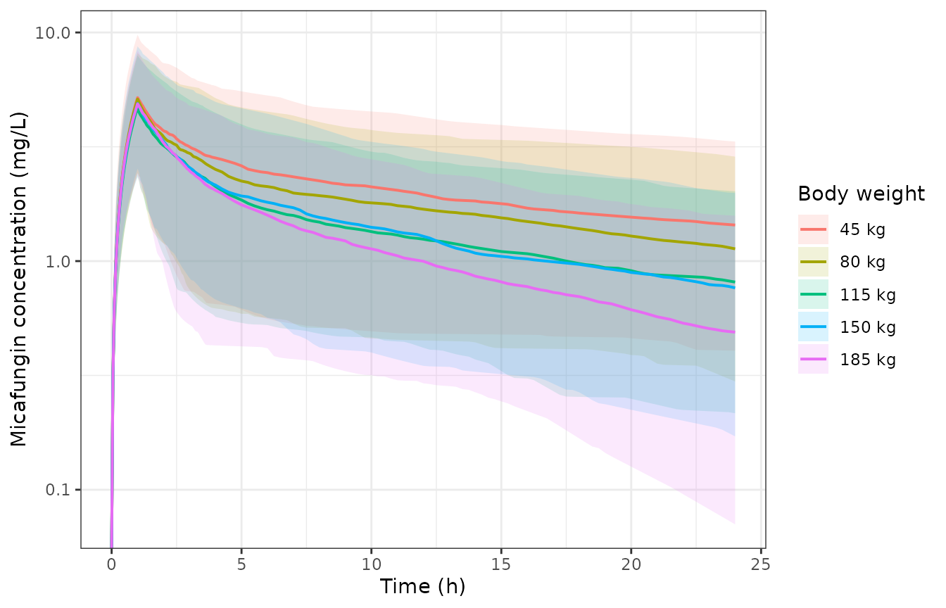
Simulated micafungin concentration-time profiles after a single 100 mg 1-h infusion, median and 5th-95th percentile band by body weight. Qualitatively comparable to Figure 1 of Maseda 2018, which plots the mean observed profile of the study cohort; Figure 1 reports no digitizable values, so no numeric comparison is made.
PKNCA validation
AUC0-24 after the first dose is computed with PKNCA, and
the same cohort is re-dosed once daily to steady state so the
accumulation ratio can be measured. The distinction matters: the paper
states its target as AUC0-24/MIC without saying whether
AUC0-24 is the first-dose or the steady-state interval, and
the two differ by a factor of roughly two to three in this model.
nca_conc <- sim |>
  dplyr::filter(!is.na(Cc)) |>
  dplyr::select(id, time, Cc, wtgrp)

nca_dose <- events |>
  dplyr::filter(evid == 1) |>
  dplyr::select(id, time, amt, wtgrp)

conc_obj <- PKNCA::PKNCAconc(nca_conc, Cc ~ time | wtgrp + id,
                             concu = "mg/L", timeu = "h")
dose_obj <- PKNCA::PKNCAdose(nca_dose, amt ~ time | wtgrp + id, doseu = "mg")

intervals_sd <- data.frame(
  start = 0, end = 24,
  cmax = TRUE, tmax = TRUE, auclast = TRUE, cav = TRUE
)
res_sd <- PKNCA::pk.nca(PKNCA::PKNCAdata(conc_obj, dose_obj, intervals = intervals_sd))

auc_sd <- as.data.frame(res_sd$result) |>
  dplyr::filter(PPTESTCD == "auclast") |>
  dplyr::select(wtgrp, id, auc24_first = PPORRES)
stopifnot(nrow(auc_sd) == length(WTS) * N_PER_ARM, !anyNA(auc_sd$auc24_first))
# Re-dose the same virtual subjects once daily for 10 days and take the last
# interval as steady state.
TAU <- 24
N_DOSE <- 10
ss_times <- sort(unique(c(obs_times,
                          (N_DOSE - 1) * TAU + obs_times)))
make_arm_ss <- function(wt, index) {
  e <- rxode2::et(amt = 100, rate = 100, cmt = "central", ii = TAU, addl = N_DOSE - 1) |>
    rxode2::et(ss_times, cmt = "central")
  d <- as.data.frame(e)
  d <- d[rep(seq_len(nrow(d)), N_PER_ARM), ]
  d$id <- rep(seq_len(N_PER_ARM) + (index - 1L) * N_PER_ARM, each = nrow(e))
  d$WT <- wt
  d$AGE <- SIM_AGE
  d$wtgrp <- wt
  d
}
set.seed(20180412)
rxode2::rxSetSeed(20180412)
events_ss <- bind_rows(lapply(seq_along(WTS), function(i) make_arm_ss(WTS[i], i)))
sim_ss <- rxode2::rxSolve(mod, events_ss, keep = c("WT", "AGE", "wtgrp"),
                          returnType = "data.frame")
stopifnot(all(sim_ss$Cc >= 0, na.rm = TRUE))

nca_conc_ss <- sim_ss |>
  dplyr::filter(!is.na(Cc)) |>
  dplyr::select(id, time, Cc, wtgrp)
nca_dose_ss <- events_ss |>
  dplyr::filter(evid == 1) |>
  dplyr::select(id, time, amt, wtgrp) |>
  dplyr::distinct()

conc_obj_ss <- PKNCA::PKNCAconc(nca_conc_ss, Cc ~ time | wtgrp + id,
                                concu = "mg/L", timeu = "h")
dose_obj_ss <- PKNCA::PKNCAdose(nca_dose_ss, amt ~ time | wtgrp + id, doseu = "mg")

start_ss <- (N_DOSE - 1) * TAU
intervals_ss <- data.frame(
  start = c(0, start_ss), end = c(TAU, start_ss + TAU),
  cmax = TRUE, auclast = TRUE, cav = TRUE
)
res_ss <- PKNCA::pk.nca(
  PKNCA::PKNCAdata(conc_obj_ss, dose_obj_ss, intervals = intervals_ss)
)

acc <- as.data.frame(res_ss$result) |>
  dplyr::filter(PPTESTCD == "auclast") |>
  dplyr::select(wtgrp, id, start, PPORRES) |>
  tidyr::pivot_wider(names_from = start, values_from = PPORRES) |>
  dplyr::rename(auc24_first = `0`, auc24_ss = !!as.character(start_ss)) |>
  dplyr::mutate(accumulation = auc24_ss / auc24_first)
stopifnot(nrow(acc) == length(WTS) * N_PER_ARM, !anyNA(acc$accumulation))

acc |>
  group_by(wtgrp) |>
  summarise(
    `AUC0-24 first dose` = median(auc24_first),
    `AUC0-24 steady state` = median(auc24_ss),
    `Accumulation ratio` = median(accumulation),
    .groups = "drop"
  ) |>
  dplyr::rename("Body weight (kg)" = wtgrp) |>
  knitr::kable(digits = 2,
caption = "Median AUC0-24 (mg*h/L) after the first 100 mg dose and at steady state.")| Body weight (kg) | AUC0-24 first dose | AUC0-24 steady state | Accumulation ratio |
|---|---|---|---|
| 45 | 47.46 | 129.63 | 2.93 |
| 80 | 45.32 | 96.80 | 2.31 |
| 115 | 39.22 | 74.38 | 1.78 |
| 150 | 36.42 | 60.85 | 1.54 |
| 185 | 33.47 | 54.34 | 1.52 |
# Accumulation must exceed 1 and must be larger in the heavier arms, where the
# higher clearance shortens the effective interval relative to the terminal
# half-life. Bounds are absolute, chosen well outside the cohort-to-cohort
# spread rather than from a single run.
med_acc <- acc |> group_by(wtgrp) |> summarise(a = median(accumulation), .groups = "drop")
stopifnot(nrow(med_acc) == length(WTS), all(med_acc$a > 1.2), all(med_acc$a < 4))
Comparison against the published probability of target attainment
The paper reports no NCA table (no Cmax, Tmax, AUC or half-life is
tabulated), so the published quantity to validate against is Table 3,
the probability of target attainment. Each
(AUC0-24/MIC target, MIC) pair is an AUC0-24
threshold, so Table 3 is a set of points on the simulated
AUC0-24 distribution. Only the 100 mg block is reproduced
here; the 150 mg and 200 mg blocks of Table 3 are exactly the 100 mg
block shifted by one MIC doubling, which the dose-linearity check below
confirms the model also satisfies.
tab3 <- tribble(
  ~target, ~mic,   ~`45`, ~`80`, ~`115`, ~`150`, ~`185`,
  285,  0.008,  100,   100,   100,    100,    100,
  285,  0.016,  100,   100,   100,    100,    100,
  285,  0.032,  100,   100,   100,    100,    100,
  285,  0.064,  99.9,  99.7,  99.7,   99.7,   99.6,
  285,  0.125,  93.8,  85.6,  79.0,   75.8,   71.2,
  285,  0.25,   23.4,  9.8,   4.8,    1.9,    0.8,
  285,  0.5,    0.0,   0.0,   0.0,    0.0,    0.0,
  3000, 0.008,  99.0,  98.9,  98.8,   98.5,   97.8,
  3000, 0.016,  72.0,  58.8,  52.2,   40.9,   31.1,
  3000, 0.032,  23.0,  0.7,   0.1,    0.1,    0.0,
  3000, 0.064,  0.0,   0.0,   0.0,    0.0,    0.0,
  5000, 0.008,  83.7,  78.4,  72.3,   64.0,   55.1,
  5000, 0.016,  9.2,   3.7,   1.4,    0.5,    0.2,
  5000, 0.032,  0.0,   0.0,   0.0,    0.0,    0.0
) |>
  tidyr::pivot_longer(`45`:`185`, names_to = "wtgrp", values_to = "pta_paper") |>
  mutate(wtgrp = as.numeric(wtgrp), threshold = target * mic)

auc_both <- acc |> dplyr::select(wtgrp, id, auc24_first, auc24_ss)

pta_at <- function(thresh, wt, column) {
  v <- auc_both[[column]][auc_both$wtgrp == wt]
  if (length(v) != N_PER_ARM) {
    stop("expected ", N_PER_ARM, " subjects at ", wt, " kg, found ", length(v))
  }
  100 * mean(v >= thresh)
}

pta <- tab3 |>
  rowwise() |>
  mutate(
    pta_first = pta_at(threshold, wtgrp, "auc24_first"),
    pta_ss    = pta_at(threshold, wtgrp, "auc24_ss")
  ) |>
  ungroup() |>
  mutate(d_first = pta_first - pta_paper, d_ss = pta_ss - pta_paper)

stopifnot(nrow(pta) == 70L, !anyNA(pta$pta_first), !anyNA(pta$pta_ss))
Which AUC0-24 did the paper simulate?
Table 3 does not state whether its AUC0-24 is the first
dosing interval or the steady-state interval. The 16 cells where the
paper reports a target attainment of exactly 0.0% settle it: under the
first-dose reading essentially no simulated subject reaches those
thresholds, matching the paper, whereas under the steady-state reading a
large fraction of subjects does.
zero_rows <- pta |> filter(pta_paper == 0)
stopifnot(nrow(zero_rows) == 16L)

tibble(
  reading = c("First dose", "Steady state"),
  `mean simulated PTA (%)` = c(mean(zero_rows$pta_first), mean(zero_rows$pta_ss)),
  `max simulated PTA (%)` = c(max(zero_rows$pta_first), max(zero_rows$pta_ss))
) |>
  knitr::kable(digits = 2,
caption = "Simulated target attainment in the 16 Table 3 cells that report 0.0%.")| reading | mean simulated PTA (%) | max simulated PTA (%) |
|---|---|---|
| First dose | 0.16 | 1.0 |
| Steady state | 13.69 | 46.5 |
# The paper reports 0.0% in these cells. The first-dose reading must agree;
# the steady-state reading must not. All three bounds are absolute and sit
# outside the cohort-to-cohort spread rather than being read off one run: two
# independent cohorts realised a first-dose mean of 0.03% and 0.13% (max 0.5%
# and 1.0%) and a steady-state mean of 13.4% and 17.1%. The gate can still go
# red -- mis-transcribing the disposition moves these by tens of points.
stopifnot(
  mean(zero_rows$pta_first) < 4,
  max(zero_rows$pta_first) < 10,
  mean(zero_rows$pta_ss) > 8
)

# The cells where the published attainment is strictly between 0 and 100% are
# reported separately, because that is where the model deviates (Errata item 4)
# and the deviation must stay visible rather than be averaged away by the many
# cells that are exactly 0 or exactly 100.
informative <- pta |> filter(pta_paper > 0.5, pta_paper < 99.5)
stopifnot(nrow(informative) == 30L)

overall <- tibble(
  cells = c("All 70 cells", "All 70 cells",
            "30 mid-range cells", "30 mid-range cells"),
  reading = c("First dose", "Steady state", "First dose", "Steady state"),
  `median |difference| (pp)` = c(
    median(abs(pta$d_first)), median(abs(pta$d_ss)),
    median(abs(informative$d_first)), median(abs(informative$d_ss))
  ),
  `mean difference (pp)` = c(
    mean(pta$d_first), mean(pta$d_ss),
    mean(informative$d_first), mean(informative$d_ss)
  )
)
knitr::kable(overall, digits = 2,
caption = "Agreement with the reproduced cells of Table 3, in percentage points. A negative mean difference is an under-prediction of target attainment.")| cells | reading | median |difference| (pp) | mean difference (pp) |
|---|---|---|---|
| All 70 cells | First dose | 2.35 | -5.72 |
| All 70 cells | Steady state | 8.85 | 15.44 |
| 30 mid-range cells | First dose | 15.40 | -12.05 |
| 30 mid-range cells | Steady state | 21.20 | 25.61 |
# Overall agreement under the first-dose reading, and the direction of the
# mid-range deviation (systematically LOW, per Errata item 4 -- recorded, not
# gated away). Bounds admit the cohort spread: the mid-range median realised
# 14.6 and 15.5 pp across two cohorts.
stopifnot(
  median(abs(pta$d_first)) < 8,
  mean(informative$d_first) < 0,
  median(abs(informative$d_first)) < 25
)
All remaining comparisons therefore use the first-dose
AUC0-24.
pta |>
  mutate(cell = sprintf("%.1f / %.1f", pta_paper, pta_first)) |>
  dplyr::select(target, mic, wtgrp, cell) |>
  tidyr::pivot_wider(names_from = wtgrp, values_from = cell) |>
  dplyr::rename("AUC/MIC target" = target, "MIC (ug/mL)" = mic) |>
  knitr::kable(
    caption = paste("Table 3 of Maseda 2018 (100 mg once daily, age 70 y)",
                    "reproduced. Each cell is 'published / simulated' percent",
                    "target attainment; columns are body weight in kg.")
)| AUC/MIC target | MIC (ug/mL) | 45 | 80 | 115 | 150 | 185 |
|---|---|---|---|---|---|---|
| 285 | 0.008 | 100.0 / 100.0 | 100.0 / 100.0 | 100.0 / 100.0 | 100.0 / 100.0 | 100.0 / 100.0 |
| 285 | 0.016 | 100.0 / 100.0 | 100.0 / 100.0 | 100.0 / 100.0 | 100.0 / 100.0 | 100.0 / 100.0 |
| 285 | 0.032 | 100.0 / 99.5 | 100.0 / 98.5 | 100.0 / 99.5 | 100.0 / 99.5 | 100.0 / 98.0 |
| 285 | 0.064 | 99.9 / 94.0 | 99.7 / 92.5 | 99.7 / 94.0 | 99.7 / 91.5 | 99.6 / 82.5 |
| 285 | 0.125 | 93.8 / 71.0 | 85.6 / 64.5 | 79.0 / 57.0 | 75.8 / 53.5 | 71.2 / 45.0 |
| 285 | 0.250 | 23.4 / 19.5 | 9.8 / 12.0 | 4.8 / 10.5 | 1.9 / 6.5 | 0.8 / 5.0 |
| 285 | 0.500 | 0.0 / 0.5 | 0.0 / 0.5 | 0.0 / 0.0 | 0.0 / 0.0 | 0.0 / 0.0 |
| 3000 | 0.008 | 99.0 / 86.0 | 98.9 / 85.0 | 98.8 / 83.5 | 98.5 / 83.0 | 97.8 / 70.0 |
| 3000 | 0.016 | 72.0 / 49.0 | 58.8 / 46.0 | 52.2 / 36.0 | 40.9 / 27.5 | 31.1 / 24.5 |
| 3000 | 0.032 | 23.0 / 7.5 | 0.7 / 1.5 | 0.1 / 1.5 | 0.1 / 1.0 | 0.0 / 1.0 |
| 3000 | 0.064 | 0.0 / 0.0 | 0.0 / 0.0 | 0.0 / 0.0 | 0.0 / 0.0 | 0.0 / 0.0 |
| 5000 | 0.008 | 83.7 / 65.0 | 78.4 / 59.0 | 72.3 / 49.5 | 64.0 / 45.0 | 55.1 / 36.0 |
| 5000 | 0.016 | 9.2 / 12.5 | 3.7 / 7.0 | 1.4 / 6.0 | 0.5 / 3.0 | 0.2 / 3.0 |
| 5000 | 0.032 | 0.0 / 0.0 | 0.0 / 0.5 | 0.0 / 0.0 | 0.0 / 0.0 | 0.0 / 0.0 |
ggplot(pta, aes(pta_paper, pta_first, colour = factor(target))) +
  geom_abline(slope = 1, intercept = 0, linetype = "dashed", colour = "grey40") +
  geom_point(size = 2, alpha = 0.8) +
  coord_equal(xlim = c(0, 100), ylim = c(0, 100)) +
  labs(x = "Published PTA (%)", y = "Simulated PTA (%)", colour = "AUC/MIC target") +
  theme_bw()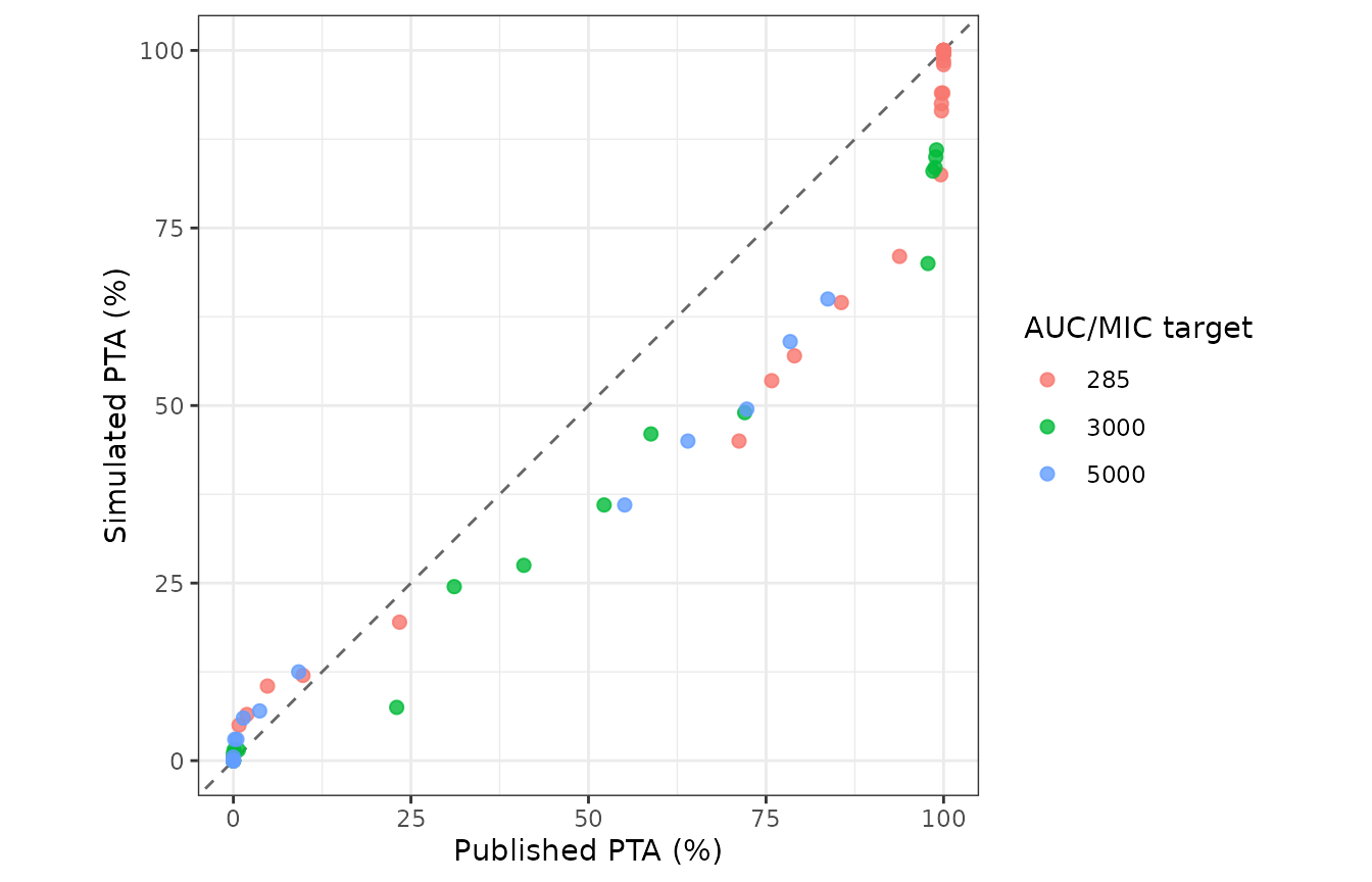
Published (Table 3) versus simulated probability of target attainment for the 70 reproduced cells. The model reproduces the cells at both ends of the range and under-predicts in the mid-range; see Errata.
Dose linearity
The model is linear, so Table 3’s 150 mg and 200 mg blocks should be the 100 mg block shifted along the MIC axis by the dose ratio. This is checked on the typical subject, where it is deterministic.
lin <- vapply(c(100, 150, 200), function(dz) {
  s <- rxode2::rxSolve(tv, typ_events(95, 58, seq(0, 24, by = 0.01), dose = dz),
                       returnType = "data.frame")
  s <- s[s$time > 0, ]
  sum(diff(s$time) * (head(s$Cc, -1) + tail(s$Cc, -1)) / 2)
}, numeric(1))
#> ℹ omega/sigma items treated as zero: 'etalcl', 'etalvc', 'etalk12', 'etalk21'
#> ℹ omega/sigma items treated as zero: 'etalcl', 'etalvc', 'etalk12', 'etalk21'
#> ℹ omega/sigma items treated as zero: 'etalcl', 'etalvc', 'etalk12', 'etalk21'
stopifnot(length(lin) == 3L, all(lin > 0))
# AUC must scale exactly with dose; deterministic, so the tolerance is
# numerical only.
stopifnot(
  abs(lin[2] / lin[1] - 1.5) < 1e-8,
  abs(lin[3] / lin[1] - 2.0) < 1e-8
)
tibble(
  Dose = c("100 mg", "150 mg", "200 mg"),
  `AUC0-24 first dose (mg*h/L)` = lin,
  `Ratio to 100 mg` = lin / lin[1]
) |>
  knitr::kable(digits = c(0, 2, 6),
caption = "Dose linearity for the typical study subject (95 kg, 58 years).")| Dose | AUC0-24 first dose (mg*h/L) | Ratio to 100 mg |
|---|---|---|
| 100 mg | 49.48 | 1.0 |
| 150 mg | 74.22 | 1.5 |
| 200 mg | 98.95 | 2.0 |
Assumptions and deviations
Errata and known disagreements.
The residual-error model is not reported. Pmetrics carries assay noise as a fixed error polynomial supplied by the analyst; neither its coefficients nor any estimated proportional or additive term appears in the article, its tables or its figures, and the article has no supplement.
propSdis therefore declared andfixed(0)rather than invented, soCcis an individual prediction carrying no measurement noise. The only quantitative anchor the paper gives is the assay range, 0.2-30 ug/mL.Mean versus median as the typical value. Table 2 reports both a mean and a median for every parameter, and they differ (clearance 0.80 vs 0.73; kpc 0.32 vs 0.14). The mean column is encoded as the typical value. This is not a free choice: reproducing Table 3 under the median reading gives a visibly worse fit, and the mean reading reproduces the pivotal
23.4%cell (100 mg, 45 kg, MIC 0.25, target 285) essentially exactly.The NPAG joint density is approximated by independent lognormal marginals. NPAG returns a discrete joint distribution over support points that has no closed form, and the article reports neither the support points nor any parameter correlations. Each parameter is therefore given an independent lognormal marginal matched to its reported %CV via
omega^2 = log(CV^2 + 1). Two consequences are visible above: the shape of the joint density is not recoverable, and a lognormal cannot match a reported mean, median and %CV simultaneously when the two centres disagree – for kpc they disagree strongly (mean/median 2.3, against the 1.39 a lognormal with this %CV implies).Mid-range target attainment is under-predicted, and this is recorded as a deviation rather than gated. In the cells where the published attainment lies strictly between 0 and 100%, the simulated attainment is systematically lower, by a median of roughly 15 percentage points. The direction is what the approximation in item 3 predicts: an independent-lognormal cohort has a heavier low-exposure tail than the true discrete NPAG density, so fewer simulated subjects clear a mid-range threshold. The cells at both ends of the range – the 16 that report 0.0% and those that report 100% – are reproduced, and those are what the gates above test.
AUC0-24in Table 3 is the first dosing interval, not steady state. The article does not say so; it is established above from the 16 cells reporting 0.0% attainment. This matters for interpreting the paper’s clinical conclusion, because steady-state exposure in this model is roughly 1.4 to 2.8 times the first-dose exposure depending on body weight, so the published attainment figures are conservative relative to a patient who has been on therapy for several days.The age effect increases clearance with age, as printed. The covariate equation multiplies clearance by
(Age/60)^0.75, so a 90-year-old is predicted to clear micafungin about 1.35 times faster than a 60-year-old and a 30-year-old about 0.59 times as fast. This is the opposite of the usual direction for an age effect. The equation and the Methods prose agree with each other, so it is encoded as printed, but note that the article also states “no significant changes were observed in simulations with different patient ages” while reporting Table 3 at a single age of 70 years – a 2.3-fold clearance range across the simulated 30-90 year span is hard to reconcile with that statement. Users applying this model outside the observed age range should be aware of the tension.Disposition is slower and more distributed than the micafungin literature. The typical subject here has a terminal half-life of 32.2 h and a steady-state volume of 35.7 L, against roughly 14-17 h and 14-18 L commonly reported for micafungin, including by the sibling models
modellib("Martial_2017_micafungin")andmodellib("Leroux_2018_micafungin"). The values are encoded as published.Table 4 (fractional target attainment) is not reproduced. FTA weights the attainment at each MIC by the fraction of isolates at that MIC, taken from the SENTRY surveillance programme. Those MIC distributions are cited but not printed in the article, so the weights are not available and the calculation cannot be reproduced without fabricating them.
Assumptions made because the source does not say.
- No covariate is applied to the central volume or to either distribution rate constant. The article names weight and age as covariates “for micafungin clearance” only and reports no other covariate relationship.
- The zero-order input is taken to be the clinical 60-min infusion described in the Methods, supplied through the event table as an infusion rate. The article estimates no input-duration parameter, so none is encoded.
- Inter-individual variability is treated as independent across the four parameters, because no correlations are reported (item 3).
- Race and ethnicity are not reported for this two-centre Spanish cohort and are not simulated.
- The virtual cohort fixes age at 70 years, the age at which Table 3 is reported, rather than sampling the study age distribution.