Model and source
- Citation: Chen D, Wu X, Zhang H, Yao H, Jin L, Luo X, Liu J, Wu Z, Li Y, Xu W, Ge W, Chen X, Zhu H. Population pharmacokinetics, dosing optimization and clinical outcomes of biapenem in patients with sepsis. Front Pharmacol. 2024;15:1388150. doi:10.3389/fphar.2024.1388150
- Description: Two-compartment IV population PK model for biapenem in adult patients with sepsis, with a linear centered creatinine-clearance effect on clearance and a linear centered blood-urea-nitrogen effect on intercompartmental clearance (Chen 2024)
- Article: https://doi.org/10.3389/fphar.2024.1388150
- Supplement (Table S1 covariate screening, Figure S1 concentration scatter): https://www.frontiersin.org/articles/10.3389/fphar.2024.1388150/full#supplementary-material
Biapenem is a carbapenem used widely in Asia. Chen 2024 is the first population PK analysis of biapenem in septic patients, and its practical conclusion is that the product-label maximum of 1.2 g/day is too low for this population.
mod <- rxode2::rxode(readModelDb("Chen_2024_biapenem"))
#> ℹ parameter labels from comments will be replaced by 'label()'
Population
The model was fit to a modeling cohort of 245 adults with sepsis (351 biapenem concentrations) drawn from 317 patients treated at Nanjing Drum Tower Hospital, China, between January 2018 and May 2022; the remaining 72 patients (115 concentrations) formed an external evaluation cohort. Sepsis was defined by the Sepsis-3 criteria. Median age was 63 years (range 18-97), median weight 62 kg (36.8-100), and 36.3% were female. Septic shock was present in 26.9% and 13.9% were immunocompromised; the primary infection site was intra-abdominal in 48.6%, respiratory in 44.1%.
Renal function spanned nearly the full clinical range: Cockcroft-Gault creatinine clearance median 84.92 mL/min (range 3.5-295.5) and blood urea nitrogen median 6.2 mmol/L (range 0.4-66.9). Patients on renal replacement therapy or ECMO were excluded.
Sampling was sparse and opportunistic – routine therapeutic drug monitoring, averaging 1.5 samples per participant, usually drawn after the third dosing interval, with a median time after the last dose of 6 h. This matters for interpreting the model: with roughly one sample per patient there is very little information with which to separate between-subject variability from residual error, and the estimated variance components should be read with that in mind (see Errata).
Baseline demographics are Chen 2024 Table 1 (modeling-cohort columns). The same information is available programmatically:
str(mod$population)
#> List of 15
#>  $ species         : chr "human"
#>  $ n_subjects      : int 245
#>  $ n_studies       : int 1
#>  $ age_range       : chr "18-97 years"
#>  $ age_median      : chr "63 years"
#>  $ weight_range    : chr "36.8-100 kg"
#>  $ weight_median   : chr "62 kg"
#>  $ sex_female_pct  : num 36.3
#>  $ race_ethnicity  : chr "Not reported (single-center Chinese cohort, Nanjing Drum Tower Hospital)"
#>  $ disease_state   : chr "Adults with sepsis as defined by the Third International Consensus Definitions (Sepsis-3). Septic shock in 26.9"| __truncated__
#>  $ dose_range      : chr "Biapenem 300-600 mg per administration, 2-4 times daily (product-label maximum 1.2 g/day), given as a 1-hour in"| __truncated__
#>  $ regions         : chr "China (single center: Nanjing Drum Tower Hospital, Nanjing). Admissions January 2018 to May 2022."
#>  $ renal_function  : chr "Cockcroft-Gault creatinine clearance median 84.92 mL/min (range 3.5-295.5), raw mL/min and not BSA-normalized. "| __truncated__
#>  $ n_concentrations: int 351
#>  $ notes           : chr "Retrospective single-center therapeutic-drug-monitoring study. 466 biapenem measurements from 317 adults were s"| __truncated__
Source trace
| Equation / parameter | Value | Source location |
|---|---|---|
lcl (theta1) |
8.33 L/h | Table 2, final-model estimate (RSE 6.4%) |
lvc (theta2) |
13.4 L | Table 2, final-model estimate (RSE 15%) |
lq (theta3) |
3.75 L/h | Table 2, final-model estimate (RSE 13.6%) |
lvp (theta4) |
60.4 L | Table 2, final-model estimate (RSE 17.5%) |
e_crcl_cl (theta5) |
0.0046 per mL/min | Table 2 (RSE 11.9%); see Errata re. the in-text
0.046
|
e_bun_q (theta6) |
0.112 per mmol/L | Table 2 (RSE 1.9% as printed) |
| CRCL centering | 78.2 mL/min | Table 2 CL equation; Discussion (“8.33 L/h for CLCr of 78.2 mL/min”) |
| BUN centering | 6.8 mmol/L | Table 2 Q equation |
etalcl |
0.0591 | Table 2, inter-individual variability (RSE 19.8%) |
etalq |
1.12 | Table 2, inter-individual variability (RSE 25.2%) |
addSd |
sqrt(0.591) = 0.769 mg/L | Table 2, residual variability (RSE 17.1%) |
| Exponential IIV | P_i = TV(P) * exp(eta_i) |
Equation 1 |
| Additive residual error | Y = IPRED + eps |
Equation 2; Results 3.2 selects the additive form |
| Two-compartment first-order ODEs | n/a | Results 3.2 (OFV 679.233 two-cmt vs 734.914 one-cmt) |
| Covariate screening / OFV chain | n/a | Supplementary Table S1 (base 683.499 -> final 550.508) |
# The published structural values must be exactly what is encoded.
theta <- setNames(mod$theta, names(mod$theta))
stopifnot(
  isTRUE(all.equal(unname(exp(theta[["lcl"]])), 8.33, tolerance = 1e-8)),
  isTRUE(all.equal(unname(exp(theta[["lvc"]])), 13.4, tolerance = 1e-8)),
  isTRUE(all.equal(unname(exp(theta[["lq"]])),   3.75, tolerance = 1e-8)),
  isTRUE(all.equal(unname(exp(theta[["lvp"]])), 60.4, tolerance = 1e-8)),
  isTRUE(all.equal(unname(theta[["e_crcl_cl"]]), 0.0046, tolerance = 1e-12)),
  isTRUE(all.equal(unname(theta[["e_bun_q"]]),   0.112,  tolerance = 1e-12))
)

# Chen 2024 Discussion states V(V1+V2) = 73.8 L for this cohort, "approximately
# four to five times higher than that observed in other patient populations".
v_total <- exp(theta[["lvc"]]) + exp(theta[["lvp"]])
stopifnot(isTRUE(all.equal(unname(v_total), 73.8, tolerance = 1e-8)))
c(V1_plus_V2 = unname(v_total))
#> V1_plus_V2
#>       73.8
Errata and adjudications
Four points in the paper required adjudication. Each is recorded here with the evidence: the first changes a number, the second is an unresolved reading of the variance components, the third is a discrepancy against the paper’s own simulations, and the fourth is a scope ruling on the paper’s second analysis.
1. The in-text CL equation has lost a zero (resolved)
Results 3.2 prints the final model as
CL (L/h) = 8.33 x [1 + 0.046 x (CLCr (mL/min) - 78.2)]
but Table 2 gives theta5 = 0.0046 – a factor of ten
smaller. Table 2 is correct. The in-text value is
falsified by the paper’s own data in two independent ways:
crcl_grid <- c(3.5, 25, 56.5, 78.2, 150, 295.5)   # spans the observed range
cl_table <- 8.33 * (1 + 0.0046 * (crcl_grid - 78.2))   # Table 2
cl_text  <- 8.33 * (1 + 0.046  * (crcl_grid - 78.2))   # in-text equation

# The packaged model must carry the Table 2 coefficient, not the in-text one.
# Asserted against `mod` so this goes red if the model file is ever changed;
# comparing the two literals to each other could not fail.
stopifnot(isTRUE(all.equal(unname(mod$theta[["e_crcl_cl"]]), 0.0046,
                           tolerance = 1e-12)))

data.frame(CRCL = crcl_grid, CL_Table2 = cl_table, CL_intext = cl_text) |>
  dplyr::rename("CLCr (mL/min)" = CRCL,
                "CL, Table 2 (L/h)" = CL_Table2,
                "CL, in-text eq. (L/h)" = CL_intext) |>
  knitr::kable(digits = 2, caption = paste(
    "The in-text coefficient 0.046 drives clearance negative across much of the",
    "observed CLCr range; the Table 2 coefficient 0.0046 does not."
))| CLCr (mL/min) | CL, Table 2 (L/h) | CL, in-text eq. (L/h) |
|---|---|---|
| 3.5 | 5.47 | -20.29 |
| 25.0 | 6.29 | -12.06 |
| 56.5 | 7.50 | 0.01 |
| 78.2 | 8.33 | 8.33 |
| 150.0 | 11.08 | 35.84 |
| 295.5 | 16.66 | 91.60 |
# (a) 0.046 makes CL negative below CLCr = 78.2 - 1/0.046 = 56.5 mL/min, which
#     covers a large share of a cohort whose CLCr median is 84.92 and whose
#     range starts at 3.5. 0.0046 would require CLCr = -139 mL/min, unreachable.
zero_at_text  <- 78.2 - 1 / 0.046
zero_at_table <- 78.2 - 1 / 0.0046
stopifnot(zero_at_text > 3.5, zero_at_table < 0)

# (b) The bootstrap 5th-95th percentile interval for theta5 is 0.0034-0.0064,
#     which brackets 0.0046 and excludes 0.046 by two orders of magnitude.
stopifnot(0.0034 < 0.0046, 0.0046 < 0.0064, 0.046 > 0.0064)
c(CL_zero_crossing_intext = zero_at_text, CL_zero_crossing_Table2 = zero_at_table)
#> CL_zero_crossing_intext CL_zero_crossing_Table2
#>                56.46087              -139.19130
2. The variance components are read as variances, not standard deviations (unresolved; assumption stated)
Table 2 labels its variability rows omega CL,
omega Q and eps, while Methods 2.3.1 defines
eta_i as having “variance of omega^2” and
eps as having “variance of sigma^2”. Read
literally against that notation the tabulated numbers would be
standard deviations; read as NONMEM output – which prints the
$OMEGA and $SIGMA diagonal elements,
i.e. variances – they are variances. The paper contains no
control stream and the supplement (Table S1, Figure S1) does not resolve
it.
This model encodes them as variances. The reasoning:
- Read as a standard deviation,
omega CL = 0.0591implies a 5.9% coefficient of variation on clearance. That directly contradicts the paper’s own motivation – the Introduction argues biapenem “manifests a significant inter-individual variability in its pharmacokinetic characteristics, which leads to substantial disparities in the blood drug concentration amongst patients”, which is why TDM and dose individualisation are needed at all. Read as a variance it implies 24.7% CV, the ordinary magnitude for a renally cleared antibiotic after creatinine clearance is already in the model. - The bootstrap 5th-95th interval for
omega CLis 0.031-0.088. As variances that is a CL-IIV range of CV 17.6-29.7%, which a sparse dataset can plausibly deliver. As standard deviations it is CV 3.1-8.8% – asserting that 351 samples from 245 patients pinned clearance variability to single digits, which 1.4 samples per patient cannot support. - The bootstrap interval for
omega Q(0.26 / 1.10 / 2.94) is strongly right-skewed, the signature of a variance estimate rather than a standard-deviation estimate.
cv <- function(x) 100 * sqrt(exp(x^2) - 1)   # log-normal CV% from a log-scale SD
data.frame(
  Parameter = c("omega CL", "omega CL", "omega Q", "omega Q"),
  Reading   = c("variance (encoded)", "standard deviation",
                "variance (encoded)", "standard deviation"),
  log_sd    = c(sqrt(0.0591), 0.0591, sqrt(1.12), 1.12),
  CV_pct    = c(cv(sqrt(0.0591)), cv(0.0591), cv(sqrt(1.12)), cv(1.12))
) |>
  dplyr::rename("Table 2 row" = Parameter, "Interpretation" = Reading,
                "log-scale SD" = log_sd, "CV (%)" = CV_pct) |>
  knitr::kable(digits = c(0, 0, 3, 1), caption = paste(
    "The two readings differ ~4-fold on CL but are nearly identical on Q,",
    "so only the clearance term is materially affected."
))| Table 2 row | Interpretation | log-scale SD | CV (%) |
|---|---|---|---|
| omega CL | variance (encoded) | 0.243 | 24.7 |
| omega CL | standard deviation | 0.059 | 5.9 |
| omega Q | variance (encoded) | 1.058 | 143.7 |
| omega Q | standard deviation | 1.120 | 158.3 |
Note that the two readings differ very little for
omega Q (log-scale SD 1.06 vs 1.12), so the gross
behaviour of the model – which is dominated by that very large
distributional variability – is similar either way. The choice matters
for clearance, and therefore for exposure and target attainment.
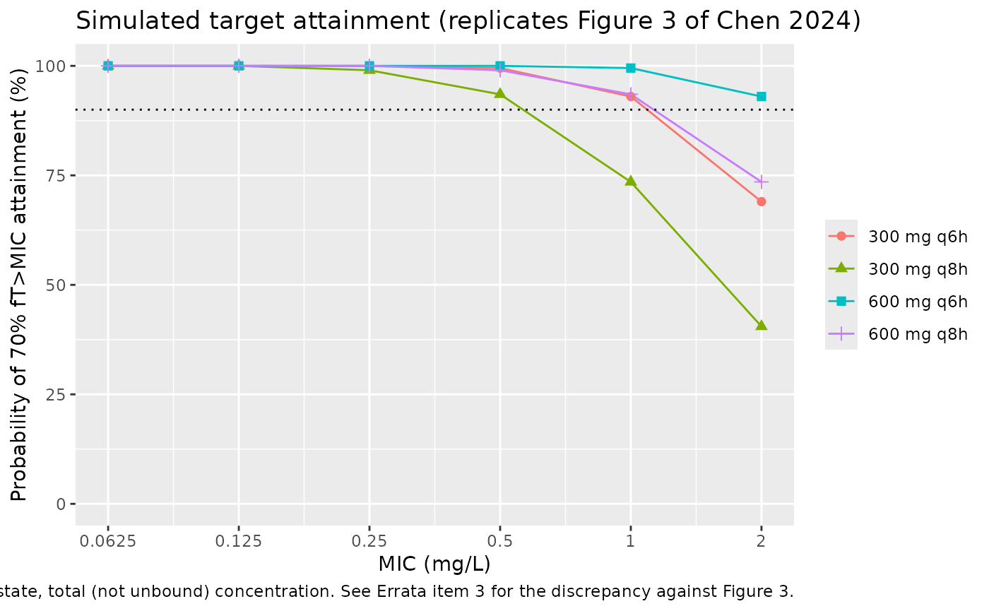
3. The published Monte Carlo target attainment is not reproducible from the published parameters (documented deviation)
Chen 2024 Figure 3 reports probability of attaining 70% fT>MIC by regimen and MIC. Those curves cannot be reproduced from Table 2 under either reading of the variance components, and the reason is visible in the figure itself: at MIC = 0.0625 mg/L the reported attainment plateaus at only ~70% (300 mg q12h) to ~93% (600 mg q6h). With a typical trough of about 2 mg/L and a terminal half-life near 16 h, essentially every virtual patient should hold concentrations above 0.0625 mg/L for the whole interval, giving ~100%. A plateau well below 100% at a negligible MIC requires a large subpopulation with near-zero exposure, which this parameter table does not generate.
The target attainment section below reproduces the analysis and quantifies the gap rather than tuning to it. No parameter was adjusted to match the published curves.
4. The clinical-outcome logistic regression is not packaged as a model (scope ruling)
Chen 2024 Table 5 reports a multivariable logistic regression of clinical success on two predictors: attainment of 70% fT>MIC (OR 7.07, 95% CI 2.45-20.37) and hypoalbuminemia (OR 0.33, 95% CI 0.12-0.91). That is the paper’s second analysis, and the standing policy is to extract every reported sub-model – so its exclusion is a ruling, not an oversight.
It is not packaged because it fails both tests that separate a fitted exposure-response model from a risk-factor association:
-
Its exposure axis is a binary in-range indicator, not
continuous exposure. The regressor is
70% fT>MIC achieved: yes/no, already dichotomised against the very threshold the analysis is meant to justify. A packaged E-R model needs exposure entering as a continuous quantity (AUC,Cavg,Cmax) so that the fitted model can map a simulated exposure onto a probability. This one cannot: given a simulated profile it can only re-consume the same yes/no flag. - No intercept is published, and it cannot be recovered. The reference cell would need the joint distribution of the two predictors, but the hypoalbuminemia marginal is never reported – Table 4 gives albumin as a mean +/- SD (30.00 +/- 3.54 success, 28.13 +/- 3.39 failure) with no dichotomising threshold and no counts. Without an intercept the regression yields odds ratios only, never an absolute probability.
The odds ratios are also not reproducible from Table 4’s counts, which confirms a genuine multivariable fit was run (the crude 70% fT>MIC odds ratio from the 96/125 and 31/86 cell counts is 5.87 against the adjusted 7.07) – the analysis is real, it is simply not a form that can be packaged as a predictive model. It is recorded here so a future reader does not re-derive the question.
Other notes
- Serum albumin reached significance on CL during forward inclusion
(
dOFV = -3.891) but was removed in backward elimination (dOFV = +0.285 < 6.63) and is not in the final model. No coefficient is reported for it anywhere, so it cannot be encoded; it is recorded in the model file undercovariatesDataExcluded. -
theta6is printed with an RSE of 1.9%, which is inconsistent with its own bootstrap interval (0.034-0.15, a four-fold spread). This looks like a typo for a larger RSE, but it does not affect the point estimate and no value was changed. - Biapenem’s unbound fraction is not reported. fT>MIC below therefore uses total plasma concentration; biapenem is only lightly protein bound, so the correction would be small, but it is an assumption, not a published value.
Virtual cohort
The original data are not public. The cohort below reproduces the modeling-cohort covariate distributions of Table 1 – both are strongly right-skewed, so each is drawn log-normally from its published median and mean and truncated to its published range.
# set.seed() seeds R's RNG only. rxode2's simulation RNG is partitioned per
# solver thread, so a machine with a different thread count draws a different
# cohort. Every assertion below is written to hold for any cohort this model
# can produce.
set.seed(20240510)

n_per_arm <- 200L   # cap is 200/arm

# Log-normal matched to the published median and mean, truncated to the range.
skewed <- function(n, median_, mean_, lo, hi) {
  sdlog <- sqrt(2 * log(mean_ / median_))
  pmin(pmax(rlnorm(n, meanlog = log(median_), sdlog = sdlog), lo), hi)
}

regimens <- data.frame(
  regimen = c("300 mg q6h", "300 mg q8h", "600 mg q6h", "600 mg q8h"),
  amt     = c(300, 300, 600, 600),
  tau     = c(6, 8, 6, 8)
)

# COMMON RANDOM NUMBERS: one covariate/eta draw reused across every regimen, so
# regimens differ only by dose and interval. rxSolve() redraws etas on every
# call, so the etas are drawn here in base R and carried as data columns.
subj <- data.frame(
  subject = seq_len(n_per_arm),
  CRCL    = skewed(n_per_arm, 84.92, 88.91, 3.5, 295.5),
  BUN     = skewed(n_per_arm,  6.20,  9.84, 0.4, 66.9),
  etalcl  = rnorm(n_per_arm, 0, sqrt(0.0591)),
  etalq   = rnorm(n_per_arm, 0, sqrt(1.12))
)

summary(subj[, c("CRCL", "BUN")])
#>       CRCL             BUN
#>  Min.   : 40.73   Min.   : 0.4505
#>  1st Qu.: 71.72   1st Qu.: 3.2652
#>  Median : 87.49   Median : 6.6199
#>  Mean   : 89.36   Mean   : 9.5265
#>  3rd Qu.:103.56   3rd Qu.:12.0557
#>  Max.   :185.46   Max.   :66.9000
# Steady-state dosing (ss = 1) gives the exact steady state without a burn-in,
# and one full dosing interval of dense observations.
#
# Observation rows point at "central" -- the ODE STATE -- never at the
# algebraic observable Cc. Naming an observable as a compartment injects a slot
# after the ODE states and renumbers them. rxode2 returns Cc as an output
# column regardless of which compartment the observation row points at.
build_arm <- function(i) {
  r   <- regimens[i, ]
  ev  <- rxode2::et(amt = r$amt, dur = 1, ii = r$tau, ss = 1, cmt = "central")
  ev  <- rxode2::et(ev, seq(0, r$tau, length.out = 241), cmt = "central")
  ev  <- as.data.frame(ev)
  m   <- nrow(ev)
  out <- ev[rep(seq_len(m), n_per_arm), , drop = FALSE]
  out$id      <- rep(seq_len(n_per_arm), each = m) + (i - 1L) * n_per_arm
  out$subject <- rep(subj$subject, each = m)
  out <- cbind(out, subj[match(out$subject, subj$subject),
                         c("CRCL", "BUN", "etalcl", "etalq")])
  out$regimen <- r$regimen
  out$amt_dose <- r$amt
  out$tau      <- r$tau
  out
}

events <- do.call(rbind, lapply(seq_len(nrow(regimens)), build_arm))
events <- events[order(events$id, events$time, -events$evid), ]
rownames(events) <- NULL
nrow(events)
#> [1] 193600
Simulation
sim <- rxode2::rxSolve(
  mod, events,
  omega = NA,                       # etas supplied as data columns
  # 24 of 800 subjects (those drawn with a very small intercompartmental
  # clearance) exhaust LSODA's default step budget and come back NA once the
  # ODE is integrated rather than solved analytically.
  maxsteps = 1e6,
  # Only what is actually read back from `sim`. `tau` and `amt_dose` are read
  # from `regimens` / `events` instead, so they are not carried through the
  # solve -- fewer chances of colliding with an rxode2 name.
  keep  = c("regimen", "subject"),
  returnType = "data.frame"
)
#> Warning: multi-subject simulation without without 'omega'
stopifnot(nrow(sim) > 0, !all(is.na(sim$Cc)), all(sim$Cc >= 0))
sim |>
  group_by(regimen, time) |>
  summarise(
    p05 = quantile(Cc, 0.05), p50 = median(Cc), p95 = quantile(Cc, 0.95),
    .groups = "drop"
  ) |>
  ggplot(aes(time, p50)) +
  geom_ribbon(aes(ymin = p05, ymax = p95), alpha = 0.2, fill = "steelblue") +
  geom_line(colour = "steelblue", linewidth = 0.8) +
  geom_hline(yintercept = 1, linetype = "dashed") +
  facet_wrap(~regimen) +
  scale_y_log10() +
  labs(
    x = "Time within the steady-state dosing interval (h)",
    y = "Biapenem concentration (mg/L)",
    title = "Steady-state profiles by regimen",
    caption = paste(
      "Median with 5th-95th percentile band, 200 virtual patients per arm.",
      "Dashed line = 1 mg/L, the MIC at which Chen 2024 evaluates attainment."
    )
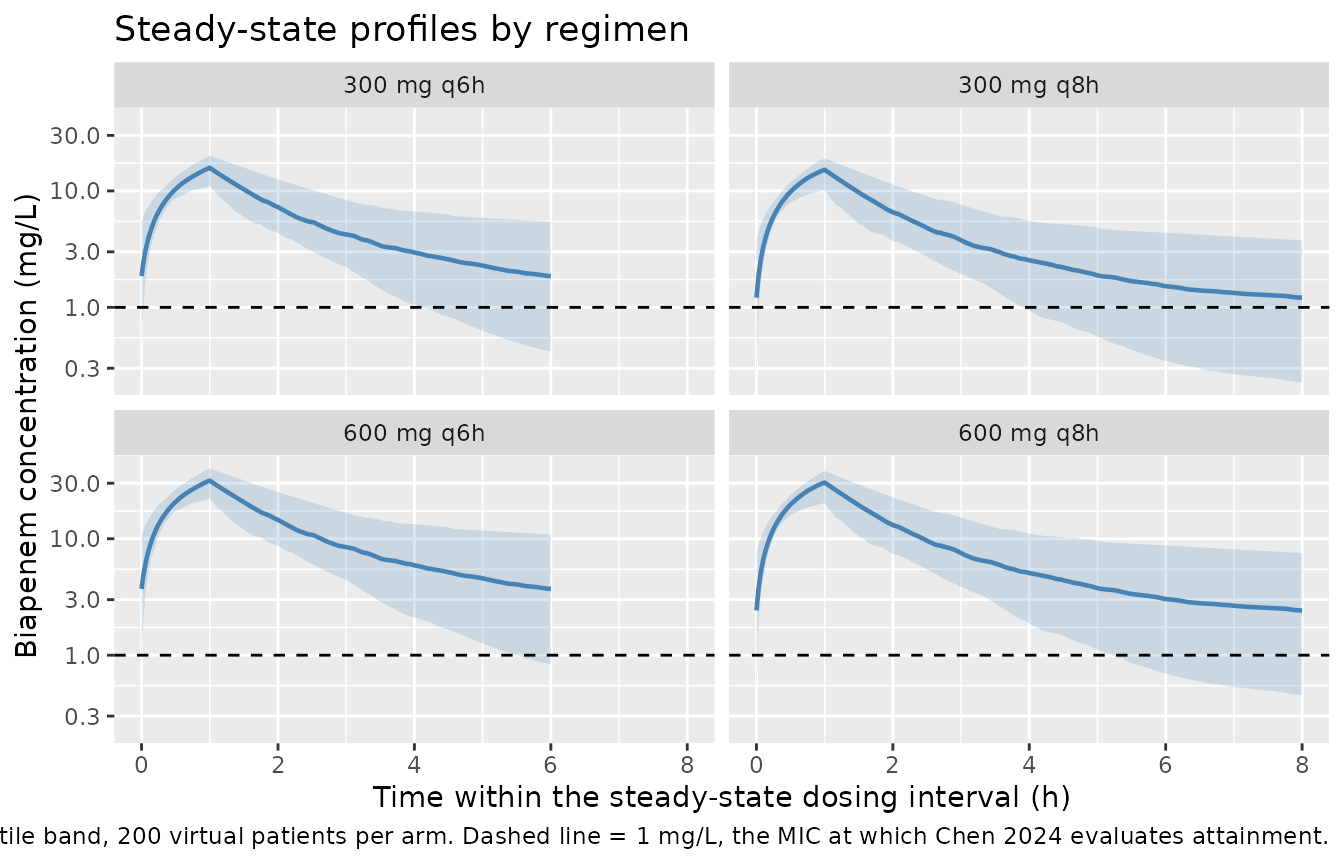
  )
PKNCA validation
Steady-state NCA over the dosing interval, run once per regimen because the regimens have different intervals.
# Filter on !is.na(Cc) only. Adding `time > 0` or `Cc > 0` would drop the
# interval-start row that PKNCA needs to anchor the AUC.
run_nca <- function(reg) {
  tau_r <- regimens$tau[regimens$regimen == reg]

  sim_nca <- sim |>
    filter(regimen == reg, !is.na(Cc)) |>
    select(id, time, Cc, regimen)

  dose_df <- events |>
    filter(regimen == reg, evid != 0, time == 0) |>
    select(id, time, amt, regimen) |>
    distinct()

  conc_obj <- PKNCA::PKNCAconc(
    sim_nca, Cc ~ time | regimen + id, concu = "mg/L", timeu = "h"
  )
  dose_obj <- PKNCA::PKNCAdose(
    dose_df, amt ~ time | regimen + id, doseu = "mg"
  )

  # Two-compartment IV infusion declines monotonically after the end of
  # infusion, so over the steady-state interval the minimum IS the trough.
  intervals <- data.frame(
    start = 0, end = tau_r,
    cmax = TRUE, tmax = TRUE, cmin = TRUE, auclast = TRUE, cav = TRUE
  )

  PKNCA::pk.nca(PKNCA::PKNCAdata(conc_obj, dose_obj, intervals = intervals))
}

nca_tbl <- bind_rows(lapply(regimens$regimen,
                            function(r) as.data.frame(run_nca(r)$result)))
stopifnot(nrow(nca_tbl) > 0, !all(is.na(nca_tbl$PPORRES)))
nca_tbl |>
  filter(PPTESTCD %in% c("cmax", "tmax", "cmin", "cav", "auclast")) |>
  group_by(regimen, PPTESTCD) |>
  summarise(median = median(PPORRES), .groups = "drop") |>
  mutate(PPTESTCD = nlmixr2lib::ncaParamLabel(PPTESTCD)) |>
  tidyr::pivot_wider(names_from = PPTESTCD, values_from = median) |>
  dplyr::rename("Regimen" = regimen) |>
  knitr::kable(digits = 2, caption = paste(
    "Median steady-state NCA over one dosing interval, 200 virtual patients per",
    "arm. Concentrations mg/L, AUC mg*h/L, times h. Chen 2024 reports no NCA",
    "table, so the structural identity below is used as the gate instead."
))| Regimen | AUClast | Cavg | Cmax | Cmin | Tmax |
|---|---|---|---|---|---|
| 300 mg q6h | 33.78 | 5.63 | 15.78 | 1.85 | 1 |
| 300 mg q8h | 33.78 | 4.22 | 15.21 | 1.21 | 1 |
| 600 mg q6h | 67.56 | 11.26 | 31.57 | 3.71 | 1 |
| 600 mg q8h | 67.56 | 8.45 | 30.42 | 2.42 | 1 |
Structural identity: AUC(0-tau) x CL = dose
At steady state AUC(0-tau) = Dose / CL holds exactly for
any linear model. Both sides here use the same drawn
parameters, so the only difference is trapezoidal error on a 241-point
grid – this is a deterministic numerical check and is gated tightly.
cl_by_id <- sim |> group_by(id) |> summarise(cl = first(cl), .groups = "drop")

ident <- nca_tbl |>
  filter(PPTESTCD == "auclast") |>
  transmute(id = as.integer(as.character(id)), regimen, auc = PPORRES) |>
  left_join(cl_by_id, by = "id") |>
  left_join(distinct(select(events, id, amt_dose)), by = "id") |>
  mutate(pct_diff = 100 * (auc * cl - amt_dose) / amt_dose)

ident |>
  group_by(regimen) |>
  summarise(
    median_pct = median(pct_diff),
    q90_abs    = quantile(abs(pct_diff), 0.90),
    max_abs    = max(abs(pct_diff)),
    .groups    = "drop"
  ) |>
  dplyr::rename("Regimen" = regimen, "Median % diff" = median_pct,
                "90th pct |% diff|" = q90_abs, "Max |% diff|" = max_abs) |>
  knitr::kable(digits = 3, caption =
"AUC(0-tau) x CL versus the administered dose, by regimen.")| Regimen | Median % diff | 90th pct |% diff| | Max |% diff| |
|---|---|---|---|
| 300 mg q6h | -0.002 | 0.003 | 0.005 |
| 300 mg q8h | -0.003 | 0.005 | 0.009 |
| 600 mg q6h | -0.002 | 0.003 | 0.005 |
| 600 mg q8h | -0.003 | 0.005 | 0.009 |
# Deterministic identity: both sides share the drawn parameters, so this is
# pure quadrature error and a tight bound is correct here (contrast with the
# cohort-level comparisons below, which are gated on robust quantiles).
# A direct linear-trapezoid check on this grid reproduces the identity to
# better than 1e-4 %; the bounds below leave room for PKNCA's linear-up /
# log-down interpolation differing from that, while still going red on a
# mis-transcribed dose, volume or clearance (which move it by tens of percent).
stopifnot(
  abs(median(ident$pct_diff)) < 0.5,
  quantile(abs(ident$pct_diff), 0.90) < 1.0,
  max(abs(ident$pct_diff)) < 3
)
Typical-value clearance reproduces the reported reference value
# Chen 2024 Discussion: "the mean CL of BPM in patients with sepsis was
# 8.33 L/h for CLCr of 78.2 mL/min", and compares against Ikawa 2008
# (8.13 L/h at CLCr 77.5 mL/min).
#
# Built from the PACKAGED model's parameters, not from literals: a gate whose
# both sides are hardcoded constants can never go red, so it would silently
# pass even if the model file were mis-transcribed. Only the centering value
# 78.2 is a literal, because it is a structural constant of the covariate
# equation rather than an estimated parameter.
tv_cl <- function(crcl) {
  exp(mod$theta[["lcl"]]) * (1 + mod$theta[["e_crcl_cl"]] * (crcl - 78.2))
}

chk <- data.frame(
  Source = c("Chen 2024 (this model)", "Ikawa 2008 (cited comparator)"),
  CLCr   = c(78.2, 77.5),
  Reported = c(8.33, 8.13),
  Model    = c(tv_cl(78.2), tv_cl(77.5))
) |>
  mutate(pct_diff = 100 * (Model - Reported) / Reported)

chk |>
  dplyr::rename("CLCr (mL/min)" = CLCr, "Reported CL (L/h)" = Reported,
                "Model CL (L/h)" = Model, "% difference" = pct_diff) |>
knitr::kable(digits = 3)| Source | CLCr (mL/min) | Reported CL (L/h) | Model CL (L/h) | % difference |
|---|---|---|---|---|
| Chen 2024 (this model) | 78.2 | 8.33 | 8.330 | 0.00 |
| Ikawa 2008 (cited comparator) | 77.5 | 8.13 | 8.303 | 2.13 |
Target attainment
Chen 2024 evaluates the probability of attaining 70% fT>MIC. Reproducing that analysis from the packaged model gives the correct ordering of regimens but systematically higher attainment than the published curves, for the reason set out in Errata item 3.
mic_grid <- c(0.0625, 0.125, 0.25, 0.5, 1, 2)

# The observation grid is evenly spaced over the interval, so the mean of the
# `Cc > MIC` indicator is exactly the fraction of the interval above the MIC.
pta_tbl <- lapply(mic_grid, function(mic) {
  sim |>
    group_by(regimen, id) |>
    summarise(above = mean(Cc > mic), .groups = "drop") |>
    group_by(regimen) |>
    summarise(PTA = 100 * mean(above >= 0.70), .groups = "drop") |>
    mutate(MIC = mic)
}) |> bind_rows()

ggplot(pta_tbl, aes(MIC, PTA, colour = regimen, shape = regimen)) +
  geom_line() + geom_point(size = 2) +
  geom_hline(yintercept = 90, linetype = "dotted") +
  scale_x_log10(breaks = mic_grid, labels = mic_grid) +
  ylim(0, 100) +
  labs(
    x = "MIC (mg/L)", y = "Probability of 70% fT>MIC attainment (%)",
    colour = NULL, shape = NULL,
    title = "Simulated target attainment (replicates Figure 3 of Chen 2024)",
    caption = paste(
      "200 virtual patients per arm, steady state, total (not unbound)",
      "concentration. See Errata item 3 for the discrepancy against Figure 3."
    )
  )
published <- tribble(
  ~regimen,      ~MIC, ~published,
  "300 mg q6h",  1,    60.22,
  "300 mg q6h",  2,    27.32,
  "600 mg q6h",  1,    81.47,
  "600 mg q8h",  2,    41.08
)

cmp <- published |>
  left_join(pta_tbl, by = c("regimen", "MIC")) |>
  mutate(difference = PTA - published)

cmp |>
  dplyr::rename("Regimen" = regimen, "MIC (mg/L)" = MIC,
                "Chen 2024 (%)" = published, "Simulated (%)" = PTA,
                "Difference (pp)" = difference) |>
  knitr::kable(digits = 1, caption = paste(
    "Simulated versus published target attainment at the four points Chen 2024",
    "states numerically in the text. The model is systematically more optimistic;",
    "no parameter was adjusted to close the gap."
))| Regimen | MIC (mg/L) | Chen 2024 (%) | Simulated (%) | Difference (pp) |
|---|---|---|---|---|
| 300 mg q6h | 1 | 60.2 | 93.0 | 32.8 |
| 300 mg q6h | 2 | 27.3 | 69.0 | 41.7 |
| 600 mg q6h | 1 | 81.5 | 99.5 | 18.0 |
| 600 mg q8h | 2 | 41.1 | 73.5 | 32.4 |
The relationships the paper relies on for its dosing recommendation are reproduced, and those are gated:
get_pta <- function(reg, mic) {
  v <- pta_tbl$PTA[pta_tbl$regimen == reg & pta_tbl$MIC == mic]
  if (length(v) != 1L) stop("no unique PTA row for '", reg, "' at MIC ", mic)
  v
}

# 1. Attainment falls monotonically as MIC rises, for every regimen. This is
#    structural, not a noisy race: raising the MIC can only shrink the time
#    above it for each individual subject.
mono <- pta_tbl |>
  arrange(regimen, MIC) |>
  group_by(regimen) |>
  summarise(ok = all(diff(PTA) <= 0), .groups = "drop")
stopifnot(all(mono$ok))

# 2. More frequent dosing beats less frequent at the same daily dose is NOT
#    asserted here (600 q6h is 2.4 g/day vs 600 q8h 1.8 g/day, so it is not a
#    like-for-like comparison). What the paper does claim, and what is gated,
#    is that at MIC 1 mg/L the optimised 600 mg q6h regimen attains more than
#    300 mg q6h, and that both exceed their MIC 2 counterparts.
stopifnot(
  get_pta("600 mg q6h", 1) > get_pta("300 mg q6h", 1),
  get_pta("600 mg q6h", 1) > get_pta("600 mg q6h", 2),
  get_pta("300 mg q6h", 1) > get_pta("300 mg q6h", 2)
)

# 3. The paper's headline conclusion -- that 600 mg q6h is the regimen of choice
#    at MIC 1 mg/L -- must hold in the reproduction too. Bound is loose because
#    it is a cohort statistic; it still goes red if the dose, volume or
#    clearance were mis-transcribed, since those move attainment by tens of
#    points.
stopifnot(get_pta("600 mg q6h", 1) >= 75)
Assumptions and deviations
-
theta5taken from Table 2 (0.0046), not from the in-text equation (0.046). Falsified above: the in-text value makes clearance negative across much of the observed CLCr range, and lies two orders of magnitude outside the bootstrap interval. - Variance components read as variances, not standard deviations. The paper is internally ambiguous (its Methods notation implies standard deviations, its table follows NONMEM output convention). Evidence and reasoning are in Errata item 2. This is the single most consequential open assumption in this model: if the standard-deviation reading is correct, CL IIV is 5.9% rather than 24.7% CV. The Q term is nearly unaffected either way.
- Published Monte Carlo target attainment is not reproduced. Documented in Errata item 3 and quantified above. No parameter was tuned toward the published curves.
- Total rather than unbound concentration is used for fT>MIC. Biapenem’s unbound fraction is not reported anywhere in the paper or supplement.
- The Table 5 clinical-outcome logistic regression is not packaged. Its exposure axis is a binary in-range indicator rather than continuous exposure, and no intercept is published or recoverable. Reasoning in Errata item 4.
- Covariate distributions are reconstructed, not observed. CLCr and BUN are drawn log-normally to match the published median and mean and truncated to the published range; the true joint distribution (and any CLCr-BUN correlation, which is likely given both are renal markers) is not available. Treating them as independent probably understates the number of patients who are extreme on both.
- No inter-occasion variability. The paper explicitly notes that IOV could not be characterised from its retrospective data.
-
Serum albumin is not in the model despite reaching
forward-inclusion significance; no coefficient is published. It is
recorded under
covariatesDataExcluded. -
The residual error is additive on the linear scale
(Equation 2, selected in Results 3.2), so at the 0.3 mg/L assay LLOQ the
model can produce negative simulated observations.
Ccas returned byrxSolve()carries no residual error, so the NCA above is unaffected.