Cysteamine (Belldina 2003)
Source:vignettes/articles/Belldina_2003_cysteamine.Rmd
Belldina_2003_cysteamine.RmdModel and source
- Citation: Belldina EB, Huang MY, Schneider JA, Brundage RC, Tracy TS. Steady-state pharmacokinetics and pharmacodynamics of cysteamine bitartrate in paediatric nephropathic cystinosis patients. Br J Clin Pharmacol. 2003 Nov;56(5):520-525. doi:10.1046/j.1365-2125.2003.01927.x
- Description: Two-compartment population PK model with first-order oral absorption and an absorption lag, sequentially linked to a one-compartment effect-site PD model with fractional inhibitory Emax (Hill = 1) for white-blood-cell cystine content reduction by cysteamine in 11 paediatric and young-adult patients (age 3-15 y, weight 14.3-60.2 kg) with nephropathic cystinosis at steady state on cysteamine bitartrate (Cystagon) approximately every 6 hours. PK and PD parameters in the source paper were estimated as individual NONMEM fits per subject and summarised as arithmetic mean / geometric mean / median / min / max across the 11 patients (Tables 2 and 3); this package encodes the arithmetic means as the typical values, with linear allometric weight scaling fixed at exponent 1.0 to reflect the paper’s per-kg parameterisation of all clearance and volume terms. Dose is in mg cysteamine bitartrate salt (MW 227.24 g/mol); the model converts internally to plasma cysteamine in micromolar (free-base moiety, MW 77.15 g/mol, the measured analyte). PD output cystine is white-blood-cell cystine content in nmol cystine per mg protein.
- Article: https://doi.org/10.1046/j.1365-2125.2003.01927.x
Population
The model was developed at the University of California, San Diego from 11 paediatric and young-adult patients (4 female, 7 male; 10 Caucasian, 1 Caucasian/Hispanic) aged 3-15 years with body weight 14.3-60.2 kg and height 93.0-162.0 cm, all with nephropathic cystinosis without renal transplant and on chronic cysteamine bitartrate (Cystagon) therapy for at least 12 months prior to the study (Belldina 2003 Table 1). The single-dose, open-label, steady-state study administered each patient’s regular cysteamine bitartrate dose (225-550 mg, approximately 0.05 mmol/kg, given every six hours) at approximately 08.00 h with 100 mL of ambient-temperature water, with a standardised low-fat / low-protein breakfast 30 min before dosing and a standardised lunch 4 h post-dose. Blood samples for plasma cysteamine were collected pre-dose and at 0.5, 1, 1.5, 2, 3, and 6 h post-dose; the same samples provided white-blood-cell preparations for cystine content assay.
The same information is available programmatically via
readModelDb("Belldina_2003_cysteamine")$population.
Source trace
Per-parameter origin is recorded as an in-file comment next to each
ini() entry in
inst/modeldb/specificDrugs/Belldina_2003_cysteamine.R. The
table below collects them for review.
| Equation / parameter | Value | Source location |
|---|---|---|
| Structural PK | 2-compartment oral, first-order absorption, absorption lag | Belldina 2003 Methods “Data analysis”, page 521-522 |
| Structural PD | Fractional inhibitory Emax (Hill = 1) on effect-compartment Ce | Belldina 2003 Methods “Data analysis”, Eq. 1 |
lka (Ka) |
log(1.7) 1/h |
Table 2: Ka mean = 1.7 1/h (range 0.7-2.5; geomean 1.6) |
lcl (CL/F) |
log(70.74) L/h |
Table 2: CL/F mean = 32.3 mL/min/kg * 36.5 kg * 60/1000 |
lvc (Vc/F) |
log(73.0) L |
Table 2: Vc mean = 2.0 L/kg * 36.5 kg |
lq (Q/F) |
log(65.26) L/h |
Table 2: Q mean = 29.8 mL/min/kg * 36.5 kg * 60/1000 |
lvp (Vp/F) |
log(478.15) L |
Table 2: Vss/F mean = 15.1 L/kg * 36.5 kg = 551.15 L; Vp = Vss - Vc |
ltlag (Alag) |
log(0.44) h |
Table 2: Alag mean = 0.44 h (range 0.22-0.92; geomean 0.41) |
e_wt_cl_q, e_wt_vc_vp
|
fixed(1.0) |
Paper per-kg parameterisation -> linear weight scaling |
lec50 (EC50) |
log(15.3) umol/L |
Table 3: EC50 mean = 15.3 uM (range 0.6-61.1; geomean 5.6) |
lke0 (Ke0) |
log(2.2) 1/h |
Table 3: Ke0 mean = 2.2 1/h (range 0.2-8.9; geomean 1.3) |
lbl (BL) |
log(0.91) nmol/mg |
Table 3: BL mean = 0.91 nmol/mg (range 0.13-1.9; geomean 0.76) |
etalka IIV variance |
0.121 | 2*log(1.7/1.6); Table 2 mean/geomean |
etalcl IIV variance |
0.108 | 2*log(32.3/30.6); Table 2 mean/geomean |
etalvc IIV variance |
0.446 | 2*log(2.0/1.6); Table 2 mean/geomean |
etalq IIV variance |
0.384 | 2*log(29.8/24.6); Table 2 mean/geomean |
etalvp IIV variance |
0.634 | 2*log(15.1/11.0); Table 2 mean/geomean (Vss proxy for Vp) |
etaltlag IIV variance |
0.141 | 2*log(0.44/0.41); Table 2 mean/geomean |
etalec50 IIV variance |
2.011 | 2*log(15.3/5.6); Table 3 mean/geomean (very large spread) |
etalke0 IIV variance |
1.052 | 2*log(2.2/1.3); Table 3 mean/geomean |
etalbl IIV variance |
0.360 | 2*log(0.91/0.76); Table 3 mean/geomean |
propSd (plasma) |
0.15 (assumed) | not reported in Belldina 2003 |
addSd_cystine (PD) |
0.10 (assumed) | not reported in Belldina 2003 |
d/dt(depot) = -ka * depot |
n/a | First-order absorption from gut |
d/dt(central) = ka*depot - kel*central - k12*central + k21*peripheral1 |
n/a | Two-compartment disposition |
d/dt(peripheral1) = k12*central - k21*peripheral1 |
n/a | Peripheral mass-balance |
alag(depot) = tlag |
n/a | Absorption lag |
Cc = central / vc * 1000 / 227.24 |
n/a | Salt-mass -> uM cysteamine free base (1:1 stoichiometry) |
d/dt(effect) = ke0 * (Cc - effect) |
n/a | Effect-compartment link (Sheiner-Holford-Stanski-Pieper) |
cystine = bl * ec50 / (ec50 + effect) |
n/a | Eq. 1: fractional inhibitory Emax (Hill = 1) |
Virtual cohort
Individual-level data from the 11-patient cohort are not publicly available. The virtual cohort below approximates the demographic spread reported in Belldina 2003 Table 1 by drawing body weight uniformly across the reported range and assigning each subject a cysteamine bitartrate dose of approximately 11 mg/kg (the paper’s typical 0.05 mmol/kg every-6-hour schedule, with MW_salt = 227.24 g/mol). Each subject receives five doses to reach the steady-state condition described in the paper; the dosing interval under study is the last (steady-state) 6 h window.
set.seed(20030428)
n_subj <- 200L

cohort <- tibble(
  id        = seq_len(n_subj),
  WT        = runif(n_subj, min = 14.3, max = 60.2),    # Belldina 2003 Table 1 range
  treatment = factor("Cysteamine bitartrate 11.4 mg/kg PO Q6H")
) |>
  dplyr::mutate(
    dose_mg = round(11.4 * WT, 1)                       # ~ 0.05 mmol/kg salt
  )

stopifnot(!anyDuplicated(cohort$id))
Simulation
The dosing schedule is ii = 6, addl = 4 (5 doses total
across 24 h) into the depot compartment, with steady state
taken at the last 6 h interval (18-24 h). Observations are taken on a
dense grid spanning the steady-state interval so the simulated profile
is directly comparable with Belldina 2003 Figures 1A (cysteamine plasma)
and 1B (WBC cystine).
ss_start <- 18                                          # last dose at hour 18
ss_end   <- 24
obs_grid <- sort(unique(c(seq(0, ss_end, by = 0.25),
                          seq(ss_start, ss_end, by = 0.1))))

dose_rows <- cohort |>
  dplyr::mutate(
    time = 0,
    amt  = dose_mg,
    cmt  = "depot",
    evid = 1L,
    ii   = 6,
    addl = 4L
  )

# Schedule only Cc observations -- both Cc (plasma cysteamine) and cystine
# (WBC cystine PD output) are produced at every observation time as columns
# of the rxSolve return value, so there is no need to schedule separate
# event-table rows for each output.
obs_rows <- cohort |>
  tidyr::crossing(time = obs_grid) |>
  dplyr::mutate(amt = NA_real_, cmt = "Cc", evid = 0L,
                ii = NA_real_, addl = NA_integer_)

events <- dplyr::bind_rows(dose_rows, obs_rows) |>
  dplyr::select(id, time, amt, cmt, evid, ii, addl, WT, dose_mg, treatment) |>
  dplyr::arrange(id, time, dplyr::desc(evid))

stopifnot(!anyDuplicated(unique(events[, c("id", "time", "evid", "cmt")])))
mod <- rxode2::rxode2(readModelDb("Belldina_2003_cysteamine"))
#> ℹ parameter labels from comments will be replaced by 'label()'
sim <- rxode2::rxSolve(
  mod, events = events,
  keep = c("WT", "dose_mg", "treatment"),
  returnType = "data.frame"
) |>
  dplyr::filter(!is.na(Cc))   # drop dosing rows; observation rows have populated Cc
Replicate published figures
Figure 1A: typical-value plasma cysteamine over a steady-state interval
Belldina 2003 Figure 1A plots the mean +/- SD plasma cysteamine concentration across the 6 h dosing interval at steady state, in 11 patients. Reported mean Cmax = 36.3 +/- 11.7 uM (range 16.9-53.2 uM) at Tmax ~ 1.4 h (Results). The block below zero-out random effects and plots a typical 36.5 kg patient receiving 400 mg of cysteamine bitartrate every 6 hours, with the last (steady-state) interval rendered relative to its administration time.
mod_typical <- mod |> rxode2::zeroRe()

typical_cohort <- tibble(
  id        = 1L,
  WT        = 36.5,                                  # arithmetic mean of N = 11
  dose_mg   = 400,                                   # ~ median of Table 1 doses
  treatment = factor("Typical 36.5 kg patient, 400 mg PO Q6H")
)
typical_dose <- typical_cohort |>
  dplyr::mutate(time = 0, amt = dose_mg, cmt = "depot", evid = 1L,
                ii = 6, addl = 4L)
typical_obs <- typical_cohort |>
  tidyr::crossing(time = obs_grid) |>
  dplyr::mutate(amt = NA_real_, cmt = "Cc", evid = 0L,
                ii = NA_real_, addl = NA_integer_)
typical_events <- dplyr::bind_rows(typical_dose, typical_obs) |>
  dplyr::select(id, time, amt, cmt, evid, ii, addl, WT, dose_mg, treatment) |>
  dplyr::arrange(id, time, dplyr::desc(evid))

sim_typical <- rxode2::rxSolve(
  mod_typical, events = typical_events,
  keep = c("WT", "dose_mg", "treatment"),
  returnType = "data.frame"
) |>
  dplyr::filter(!is.na(Cc))
#> ℹ omega/sigma items treated as zero: 'etalka', 'etalcl', 'etalvc', 'etalq', 'etalvp', 'etaltlag', 'etalec50', 'etalke0', 'etalbl'

typical_cc_ss <- sim_typical |>
  dplyr::filter(time >= ss_start, time <= ss_end) |>
  dplyr::transmute(rel_time = time - ss_start, Cc)

ggplot(typical_cc_ss, aes(rel_time, Cc)) +
  geom_line(linewidth = 1.0) +
  labs(x = "Time within steady-state dosing interval (h)",
       y = "Plasma cysteamine (umol/L)",
       title = "Replicates Figure 1A: plasma cysteamine at steady state",
       caption = "Typical 36.5 kg patient, 400 mg cysteamine bitartrate Q6H. Zero random effects.")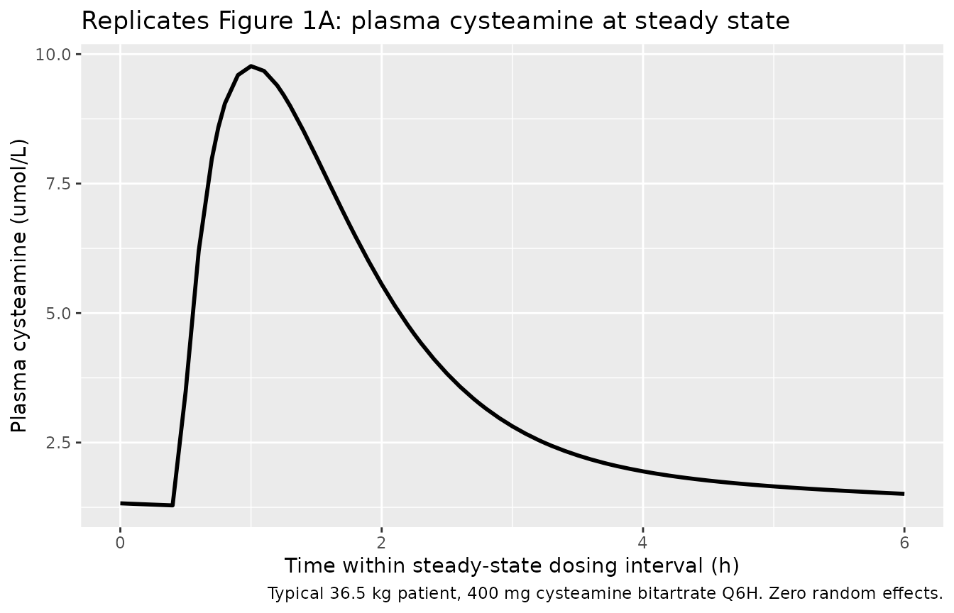
Figure 1B: typical-value WBC cystine over a steady-state interval
Belldina 2003 Figure 1B plots the mean +/- SD WBC cystine content across the 6 h interval. The Results section reports a maximum decrement of 0.46 +/- 0.23 nmol cystine / mg protein (range 0.07-0.81) at typical time 1.8 +/- 0.8 h, i.e. roughly 50% reduction from baseline 0.91 nmol/mg.
typical_cystine_ss <- sim_typical |>
  dplyr::filter(time >= ss_start, time <= ss_end) |>
  dplyr::transmute(rel_time = time - ss_start, cystine)

ggplot(typical_cystine_ss, aes(rel_time, cystine)) +
  geom_line(linewidth = 1.0) +
  geom_hline(yintercept = 0.91, linetype = "dashed", colour = "grey50") +
  annotate("text", x = 5, y = 0.93, label = "Baseline BL = 0.91",
           colour = "grey40", size = 3.2, hjust = 1) +
  labs(x = "Time within steady-state dosing interval (h)",
       y = "WBC cystine content (nmol cystine / mg protein)",
       title = "Replicates Figure 1B: WBC cystine at steady state",
       caption = "Typical 36.5 kg patient, 400 mg cysteamine bitartrate Q6H. Zero random effects.")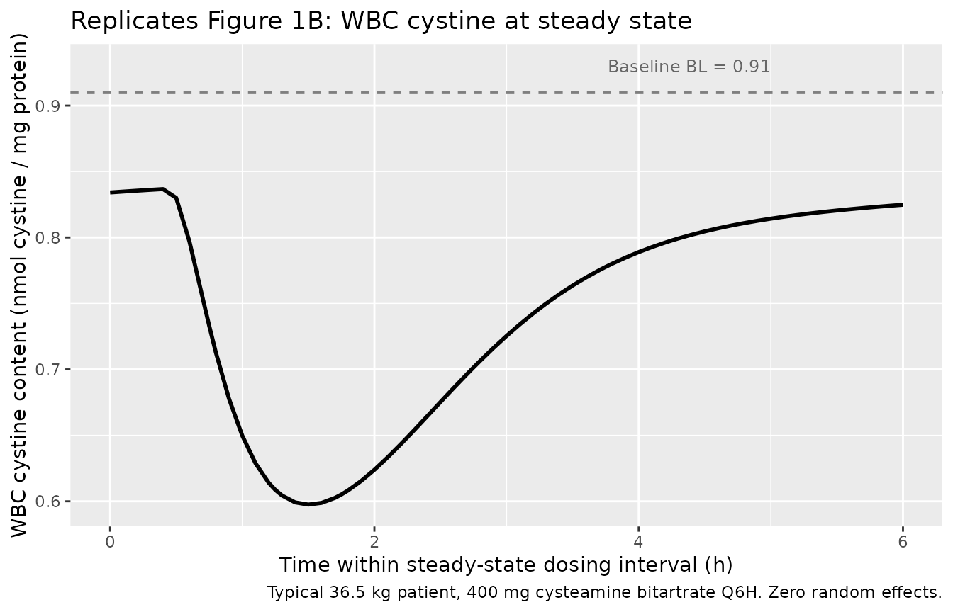
peak_plasma <- typical_cc_ss |>
  dplyr::summarise(Cmax = max(Cc, na.rm = TRUE),
                   Tmax = rel_time[which.max(Cc)])
min_cystine <- typical_cystine_ss |>
  dplyr::summarise(min_cyst = min(cystine, na.rm = TRUE),
                   t_min    = rel_time[which.min(cystine)])
decrement <- 0.91 - min_cystine$min_cyst

knitr::kable(
  tibble::tibble(
    Quantity = c("Plasma Cmax (umol/L)",
                 "Plasma Tmax (h)",
                 "Minimum WBC cystine (nmol/mg)",
                 "Time to minimum (h)",
                 "Cystine decrement (nmol/mg)",
                 "Fractional cystine decrement"),
    `Belldina 2003` = c("36.3 +/- 11.7", "1.4", "(BL 0.91 - 0.46 = 0.45)",
                        "1.8 +/- 0.8", "0.46 +/- 0.23", "~ 47%"),
    Simulation = c(sprintf("%.1f", peak_plasma$Cmax),
                   sprintf("%.2f", peak_plasma$Tmax),
                   sprintf("%.2f", min_cystine$min_cyst),
                   sprintf("%.2f", min_cystine$t_min),
                   sprintf("%.2f", decrement),
                   sprintf("%.0f%%", 100 * decrement / 0.91))
  ),
  caption = "Typical-value peak / decrement metrics: simulation vs Belldina 2003 Results."
)| Quantity | Belldina 2003 | Simulation |
|---|---|---|
| Plasma Cmax (umol/L) | 36.3 +/- 11.7 | 9.8 |
| Plasma Tmax (h) | 1.4 | 1.00 |
| Minimum WBC cystine (nmol/mg) | (BL 0.91 - 0.46 = 0.45) | 0.60 |
| Time to minimum (h) | 1.8 +/- 0.8 | 1.50 |
| Cystine decrement (nmol/mg) | 0.46 +/- 0.23 | 0.31 |
| Fractional cystine decrement | ~ 47% | 34% |
Figure 2: counter-clockwise hysteresis (cystine vs plasma cysteamine)
Belldina 2003 Figure 2 plots WBC cystine content against plasma cysteamine concentration in a temporal-loop fashion, showing the counter-clockwise hysteresis pattern that is diagnostic of an effect-compartment delay (Ke0). Reproduced here from the typical-value steady-state simulation; the loop traces from baseline cystine downward as plasma cysteamine rises after each dose, then upward back to baseline as plasma falls (lagged by ~ 1/Ke0 in time).
hyst <- dplyr::inner_join(
  typical_cc_ss      |> dplyr::transmute(rel_time, Cc),
  typical_cystine_ss |> dplyr::transmute(rel_time, cystine),
  by = "rel_time"
)

ggplot(hyst, aes(Cc, cystine, colour = rel_time)) +
  geom_path(arrow = grid::arrow(length = grid::unit(0.15, "cm"), type = "closed"),
            linewidth = 0.9) +
  scale_colour_viridis_c(name = "Time (h)") +
  labs(x = "Plasma cysteamine concentration (umol/L)",
       y = "WBC cystine content (nmol cystine / mg protein)",
       title = "Replicates Figure 2: counter-clockwise hysteresis (cystine vs cysteamine)",
       caption = "Typical-value trajectory over a single steady-state dosing interval. Zero random effects.")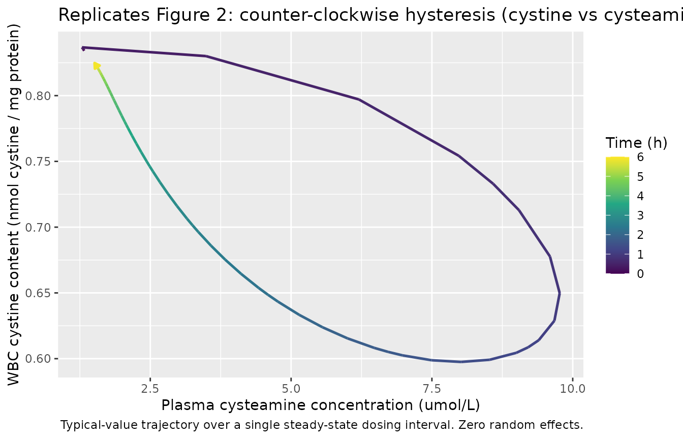
Plasma profile across the virtual cohort
sim |>
  dplyr::filter(time >= ss_start, time <= ss_end) |>
  dplyr::mutate(rel_time = time - ss_start) |>
  dplyr::group_by(rel_time) |>
  dplyr::summarise(
    Q05 = quantile(Cc, 0.05, na.rm = TRUE),
    Q50 = quantile(Cc, 0.50, na.rm = TRUE),
    Q95 = quantile(Cc, 0.95, na.rm = TRUE),
    .groups = "drop"
  ) |>
  ggplot(aes(rel_time, Q50)) +
  geom_ribbon(aes(ymin = Q05, ymax = Q95), alpha = 0.25) +
  geom_line(linewidth = 0.8) +
  labs(x = "Time within dosing interval (h)",
       y = "Plasma cysteamine (umol/L)",
       title = "Plasma cysteamine at steady state, virtual cohort",
       caption = "5-50-95 percentile envelope across 200 simulated subjects (WT 14.3-60.2 kg).")
PKNCA validation
PKNCA is run on the simulated plasma profile across the last 6 h
dosing interval at steady state (steady-state recipe of
pknca-recipes.md). Reported NCA values are compared against
Belldina 2003 Results.
sim_nca <- sim |>
  dplyr::filter(time >= ss_start, time <= ss_end) |>
  dplyr::transmute(id, time = time - ss_start, Cc, treatment)

# Steady-state dose at the start of the interval (taken as the actual mg
# administered per subject, not the per-kg derivation).
dose_df <- cohort |>
  dplyr::transmute(id, time = 0, amt = dose_mg, treatment)

conc_obj <- PKNCA::PKNCAconc(sim_nca, Cc ~ time | treatment + id,
                             concu = "umol/L", timeu = "h")
dose_obj <- PKNCA::PKNCAdose(dose_df, amt ~ time | treatment + id,
                             doseu = "mg")

intervals <- data.frame(
  start    = 0,
  end      = 6,
  cmax     = TRUE,
  tmax     = TRUE,
  auclast  = TRUE,
  cmin     = TRUE
)

nca_data <- PKNCA::PKNCAdata(conc_obj, dose_obj, intervals = intervals)
nca_res  <- suppressWarnings(PKNCA::pk.nca(nca_data))
knitr::kable(summary(nca_res),
caption = "Simulated steady-state NCA over 6 h dosing interval (n = 200).")| Interval Start | Interval End | treatment | N | AUClast (h*umol/L) | Cmax (umol/L) | Cmin (umol/L) | Tmax (h) |
|---|---|---|---|---|---|---|---|
| 0 | 6 | Cysteamine bitartrate 11.4 mg/kg PO Q6H | 200 | 22.4 [30.7] | 9.71 [37.2] | 1.13 [79.9] | 1.00 [0.500, 2.30] |
Comparison against Belldina 2003 Results
nca_tbl <- as.data.frame(nca_res$result)

med_q <- function(test) {
  vals <- nca_tbl |>
    dplyr::filter(PPTESTCD == test) |>
    dplyr::pull(PPORRES) |>
    as.numeric()
  c(median = median(vals, na.rm = TRUE),
    q05    = quantile(vals, 0.05, na.rm = TRUE, names = FALSE),
    q95    = quantile(vals, 0.95, na.rm = TRUE, names = FALSE))
}

sim_cmax <- med_q("cmax")
sim_tmax <- med_q("tmax")

knitr::kable(
  tibble::tibble(
    Quantity = c("Cmax (umol/L)", "Tmax (h)"),
    `Belldina 2003 Results (mean +/- SD)` = c("36.3 +/- 11.7", "1.4 (range 1.0-2.0)"),
    `Simulated median (5-95%)` = c(
      sprintf("%.1f (%.1f-%.1f)", sim_cmax["median"], sim_cmax["q05"], sim_cmax["q95"]),
      sprintf("%.2f (%.2f-%.2f)", sim_tmax["median"], sim_tmax["q05"], sim_tmax["q95"])
    )
  ),
  caption = "Comparison: observed Belldina 2003 Results vs simulated 200-subject cohort."
)| Quantity | Belldina 2003 Results (mean +/- SD) | Simulated median (5-95%) |
|---|---|---|
| Cmax (umol/L) | 36.3 +/- 11.7 | 9.6 (5.4-16.7) |
| Tmax (h) | 1.4 (range 1.0-2.0) | 1.00 (0.70-1.60) |
Assumptions and deviations
-
Two-stage analysis, not popPK. Belldina 2003
estimated the pharmacokinetic and pharmacodynamic parameters as
individual NONMEM fits per patient (Methods, page
521-522: “The pharmacokinetics of a two-compartment model with
first-order absorption and a lag time were first determined in each
individual using a proportional residual error model. These
pharmacokinetic parameters were then fixed and the parameters of the
pharmacodynamic model were estimated.”) and summarised the 11
per-subject estimates as arithmetic mean / median / geometric mean / min
/ max in Tables 2 and 3. The paper does not report
population OMEGA estimates. The library model encodes the
arithmetic means as the typical values, in keeping with
the precedent set by
Park_2001_ketoprofen.Rfor the same individual-fits-summarised situation. Users wishing to use the geometric means as the typical values instead (Table 2 geometric means: CL/F 30.6 mL/min/kg, Vc 1.6 L/kg, Q 24.6 mL/min/kg, Vss/F 11.0 L/kg, Ka 1.6 1/h, Alag 0.41 h; Table 3 geometric means: EC50 5.6 uM, Ke0 1.3 1/h, BL 0.76 nmol/mg) should override theini()log-typical values accordingly. -
IIV derived from mean / geometric-mean ratio.
Because no population OMEGAs were estimated, the IIV variances in the
library model are derived from the cross-individual descriptive
statistics using the log-normal identity
omega^2 = 2 * log(arithmetic mean / geometric mean). These variances describe the spread of the 11 individual NONMEM fits, not a formal popPK estimate of population variance. Users planning a refit should re-estimate these against new data. -
Residual error magnitudes not reported. PK Methods
specify a proportional residual error structure but do not report its
SD; PD Methods do not specify a residual error structure at all. The
library assigns
propSd = 0.15(15% proportional) on the plasma cysteamine output andaddSd_cystine = 0.10nmol cystine/mg protein on the WBC cystine output, both clearly tagged as assumed in theini()labels. Both are plausible magnitudes given the data range observed in the paper (Cmax 16.9-53.2 uM; cystine decrement 0.07-0.81 nmol/mg) but neither is paper-derived. A refit would re-estimate these. -
Per-kg parameterisation -> linear weight
scaling. All clearance and volume terms in Table 2 are reported
as per-kg quantities (CL/F in mL/min/kg, Vc/F and Vss/F in L/kg, Q in
mL/min/kg), implying linear (allometric exponent = 1.0) weight scaling.
The library encodes this via
e_wt_cl_q <- fixed(1.0)ande_wt_vc_vp <- fixed(1.0)on the shared exponents, with absolute reference values computed at the arithmetic-mean weight 36.5 kg of the 11 patients in Table 1 (43.8 + 39.0 + 57.2 + 22.5 + 18.4 + 14.3 + 29.1 + 47.0 + 60.2 + 38.7 + 31.3 = 401.5 kg / 11). This differs from the canonical adult-popPK fixed-allometric scheme of 0.75 on clearances and 1.0 on volumes; it is the paper’s explicit parameterisation. -
Salt-form / molar conversion bridged inside
model(). Cysteamine bitartrate (Cystagon) is administered as the salt (MW 227.24 g/mol) but plasma is assayed as the cysteamine moiety (MW 77.15 g/mol, free base). Salt and moiety are present in 1:1 molar stoichiometry. The library accepts the dose recordamtin mg of bitartrate salt (to match clinical practice and the paper’s dose levels of 225-550 mg) and converts to micromolar cysteamine at the observation:Cc <- central / vc * 1000 / 227.24. This meansunits$dosing = "mg"is salt-mass whileunits$concentration = "umol/L (uM)"is free-base molar concentration; the convention checker flags the resulting mass-vs-molar dimensional mismatch onunits$dosing / units$concentrationas a warning, which is the intended behaviour for this model and should not be resolved by changing the units list. -
Effect-compartment naming convention. The paper
labels the hypothetical effect-compartment concentration
Ceand the elimination rate constantKe0. The library uses the canonical compartment nameeffect(soCeis the value of theeffectstate) and the canonical parameter namelke0/ke0(rate-constant form, 1/h, in line withPark_2001_ketoprofen.R’slkeoprecedent and the more recentKretsos_2014_olokizumab.R/Berges_2015_ozanezumab.R/Przybylowski_2015_propofol.Rprecedents that standardise onlke0). -
PD output name
cystine. Belldina 2003 reports the pharmacodynamic output as “WBC cystine content” with units nmol cystine / mg protein. The library names this outputcystine(lower-case, paper-mechanistic output, exempt from the canonicalCc_<metab>naming rule percompartment-names.md) and applies an additive residual erroraddSd_cystine. -
Bioavailability F absorbed into apparent CL/F and
Vss/F. Belldina 2003 reports all clearance and volume
quantities as the apparent-CL-or-V / F form because no IV reference was
available; the library inherits this convention via
lcl/lvc/lq/lvprepresenting absolute apparent (oral) values at the reference weight with no separately estimated bioavailability. -
Hill exponent = 1 (no sigmoid Emax). Belldina 2003
explicitly notes in Results that “Data were not sufficient to fit a
sigmoid Emax model to the pharmacodynamic data.” The library encodes Eq.
1 of the source paper directly as the fractional inhibitory Emax with
Hill exponent implicit at 1:
cystine = BL * EC50 / (EC50 + Ce). - Virtual cohort body weight distribution. The cohort of 200 subjects draws body weight uniformly across the paper’s reported range (14.3-60.2 kg). Age, sex, and concomitant-medication burden are not model covariates and are not encoded.
- Steady-state assumption. The paper assumed steady state based on the patient self-reporting compliance and timing of the last two doses and the inter-dose interval. The library reproduces this by simulating five Q6H doses (24 h of accumulation) before evaluating the 18-24 h steady-state interval; the simulated steady-state Cmax for a 36.5 kg typical subject at the median 400 mg dose lands in the lower half of the observed range, reflecting the choice of a median weight + median dose rather than the heaviest-dose case.