Dextromethorphan whole-body PBPK and CYP2D6 phenotyping (Grzegorzewski 2022)
Source:vignettes/articles/Grzegorzewski_2022_dextromethorphan_pbpk.Rmd
Grzegorzewski_2022_dextromethorphan_pbpk.RmdThe model
Grzegorzewski_2022_dextromethorphan_pbpk is the
whole-body physiologically based pharmacokinetic (PBPK) model of
dextromethorphan (DXM) that Grzegorzewski, Brandhorst and Koenig (2022)
built to study CYP2D6 metabolic phenotyping. It tracks DXM, its CYP2D6
O-demethylation product dextrorphan (DXO), and dextrorphan O-glucuronide
(DXO-Glu) through a nine-organ body and predicts the urinary cumulative
metabolic ratio
that is used clinically to classify subjects as poor (PM), intermediate (IM), extensive (EM), or ultrarapid (UM) metabolizers.
The authors distribute the model as SBML (version 0.9.5, the version
used in the paper). Because the paper does not print its rate laws, the
maintainers ported them from that archive (doi:10.5281/zenodo.7025683,
models/dextromethorphan_body_flat.xml) and checked the port
reproduces the archive exactly (see “Reproducing the deposited SBML
model” below).
mod <- rxode2::rxode2(readModelDb("Grzegorzewski_2022_dextromethorphan_pbpk"))
length(mod$state)
#> [1] 76
The 76 states are concentrations (mmol/L) for each of DXM, DXO and
DXO-Glu in the plasma and tissue sub-spaces of gut, pancreas, spleen,
portal vein, liver, hepatic vein, kidney, lung, forearm and a lumped
rest-of-body compartment, plus the venous and arterial blood pools; two
dosing compartments (depot oral, depot_iv
intravenous, both mg); the gut lumen and feces; and the three urinary
excretion pools.
-
Absorption. Oral DXM dissolves from
depotinto the gut lumen; 55% of the dissolved dose is absorbed into gut tissue and 45% is excreted in feces. Gut-wall CYP3A4 removes part of the absorbed DXM (first-pass N-demethylation). -
Circulation. Gut, pancreas and spleen drain to the
portal vein; the portal vein and hepatic artery perfuse the liver, which
drains through the hepatic vein. Kidney, lung, forearm and the rest
compartment exchange with their plasma spaces by tissue/plasma partition
coefficients. Plasma is sampled at the forearm (median cubital) vein, so
the observations
Cc,Cc_dxorandCc_dxorglucread the forearm-vein concentration (nmol/L). - Metabolism. In the liver DXM is O-demethylated to DXO by CYP2D6 (main route) and CYP3A4 (minor route), and DXO is glucuronidated to DXO-Glu by UGT. All are irreversible Michaelis-Menten reactions scaled by functional liver tissue volume.
-
CYP2D6 activity score. The covariate
CYP2D6is the activity score (AS, 0–4) summed from the subject’s diplotype. The CYP2D6 Vmax is proportional to AS and the Km is multiplied byAS^lambda_1(lambda_1= -0.4), so a higher AS means a faster and higher-affinity CYP2D6.AS = 0removes the CYP2D6 pathway, leaving only the minor CYP3A4 O-demethylation. - Between-subject variability. Hepatic CYP2D6 and CYP3A4 Km and Vmax carry a correlated log-normal distribution fitted to human liver microsome data; this is the sole source of the UCMR dispersion.
Population
pop <- attr(readModelDb("Grzegorzewski_2022_dextromethorphan_pbpk"), "population")
str(pop, max.level = 1)
#>  NULL
The model was calibrated against concentration-time and urinary data from 36 clinical studies curated into PK-DB (Table 1 of the paper), covering oral doses from 2 mg to 3 mg/kg (most commonly 30 mg) and one intravenous study. Subjects are healthy adults spanning European, East Asian, Mexican Mestizo, Cuban and Trinidadian cohorts.
Source trace
Every parameter in the model file carries an in-line comment pointing to its source location. The table below summarises the provenance of the model’s structural equations and the parameters whose values drive the figures.
| Component | Source location |
|---|---|
| Whole-body circulation ODEs, organ volumes, blood flows, blood-pool corrections | Zenodo 7025683 dextromethorphan_body_flat.xml;
summarised in Table 2 and Figure 1 |
Partition coefficients kp_*, tissue rates
ftissue_* (fitted) |
Table 2 (flag F) |
Absorption ka_abs_dxm, fraction absorbed
f_dxm_abs = 0.55 |
Table 2; Schadel 1995 |
Dissolution ka_dis_dxm (unit reinterpreted, see
Errata) |
Table 2 Ka_dis_dxm
|
Hepatic CYP2D6 Vmax / Km, lambda_1 = -0.4 |
Table 2; Figure 2B; Storelli 2019a, Yang 2012 |
| Hepatic CYP3A4 Vmax / Km | Table 2; Yu 2001 |
| UGT Vmax / Km | Table 2; Lutz 2012 |
| Gut CYP3A4 Vmax / Km | Table 2; Kerry 1994, Yu 2001 |
Renal excretion kex_* (fitted) |
Table 2 |
| CYP2D6 activity-score means (Vmax, Km per AS) | Figure 2B table |
| Between-subject Km/Vmax dispersion and correlation | Figure 2A (CYP3A4), Figure 2B panels (CYP2D6) – digitised |
Simulation helpers
# Typical-value model: zero out the enzyme IIV for deterministic replications.
mod_typ <- rxode2::zeroRe(mod)

# An oral event table at a chosen dose and activity score.
oral_events <- function(as, dose_mg = 30, tmax = 1440, by = 15) {
  rxode2::et(amt = dose_mg, cmt = "depot") |>
    rxode2::et(seq(0, tmax, by = by)) |>
    as.data.frame() |>
    dplyr::mutate(WT = 75, CYP2D6 = as)
}
Reproducing the deposited SBML model
The authoritative check for a ported PBPK model is that it reproduces
the deposited model it was ported from. The reference values below were
produced by simulating the archive’s
dextromethorphan_body_flat.xml under libRoadRunner (a 75 kg
subject, 30 mg oral DXM, the diplotype fixed to activity score 0, 1 or
2) and reading the forearm-vein DXM and DXO concentrations (nmol/L) and
the urinary UCMR. The port must match them to within solver
tolerance.
# forearm-vein DXM (nmol/L), DXO (nmol/L) and urinary UCMR from the archive,
# at t = 30, 120, 240, 480, 720, 1440 min.
ref_times <- c(30, 120, 240, 480, 720, 1440)
reference <- tibble::tribble(
  ~CYP2D6, ~time,  ~dxm_ref,  ~dxo_ref, ~ucmr_ref,
  0,   30, 16.7919,  0.0688, 2.92537,
  0,  120, 69.3951,  0.4055, 1.39728,
  0,  240, 66.6061,  0.3590, 1.21942,
  0,  480, 62.3086,  0.2542, 1.39859,
  0,  720, 58.5806,  0.2108, 1.55287,
  0, 1440, 48.7698,  0.1630, 1.77752,
  1,   30,  5.8978,  3.4445, 0.01971,
  1,  120, 12.7608, 10.8334, 0.00959,
  1,  240, 10.0173,  7.3587, 0.00860,
  1,  480,  6.5547,  2.9572, 0.01031,
  1,  720,  4.3164,  1.3150, 0.01179,
  1, 1440,  1.2368,  0.2108, 0.01378,
  2,   30,  2.7130,  4.3353, 0.00718,
  2,  120,  5.2281, 12.1496, 0.00348,
  2,  240,  4.0123,  7.9310, 0.00315,
  2,  480,  2.5042,  2.8827, 0.00382,
  2,  720,  1.5735,  1.1084, 0.00439,
  2, 1440,  0.3918,  0.1032, 0.00514
)

port <- lapply(c(0, 1, 2), function(as) {
  s <- rxode2::rxSolve(mod_typ, oral_events(as, by = 10), returnType = "data.frame")
  s <- s[s$time %in% ref_times, c("time", "Cc", "Cc_dxor", "UCMR")]
  s$CYP2D6 <- as
  s
})
#> ℹ omega/sigma items treated as zero: 'etalvmax2d6', 'etalkm2d6', 'etalvmax3a4', 'etalkm3a4'
#> ℹ omega/sigma items treated as zero: 'etalvmax2d6', 'etalkm2d6', 'etalvmax3a4', 'etalkm3a4'
#> ℹ omega/sigma items treated as zero: 'etalvmax2d6', 'etalkm2d6', 'etalvmax3a4', 'etalkm3a4'
port <- do.call(rbind, port)

cmp <- merge(reference, port, by = c("CYP2D6", "time"))
cmp <- cmp[order(cmp$CYP2D6, cmp$time), ]
cmp$dxm_pct <- 100 * (cmp$Cc - cmp$dxm_ref) / cmp$dxm_ref
cmp$ucmr_pct <- 100 * (cmp$UCMR - cmp$ucmr_ref) / cmp$ucmr_ref

# The port must reproduce the archive essentially exactly.
stopifnot(
  max(abs(cmp$dxm_pct)) < 0.5,
  max(abs(cmp$ucmr_pct)) < 0.5
)
round(
  cmp[, c("CYP2D6", "time", "Cc", "dxm_ref", "dxm_pct", "UCMR", "ucmr_ref", "ucmr_pct")],
  4
) |>
  dplyr::rename(
    "AS" = CYP2D6, "Time (min)" = time,
    "DXM port" = Cc, "DXM archive" = dxm_ref, "DXM % diff" = dxm_pct,
    "UCMR port" = UCMR, "UCMR archive" = ucmr_ref, "UCMR % diff" = ucmr_pct
  ) |>
knitr::kable()| AS | Time (min) | DXM port | DXM archive | DXM % diff | UCMR port | UCMR archive | UCMR % diff | |
|---|---|---|---|---|---|---|---|---|
| 4 | 0 | 30 | 16.7919 | 16.7919 | -0.0002 | 2.9254 | 2.9254 | -0.0004 |
| 1 | 0 | 120 | 69.3952 | 69.3951 | 0.0001 | 1.3973 | 1.3973 | -0.0002 |
| 3 | 0 | 240 | 66.6061 | 66.6061 | 0.0000 | 1.2194 | 1.2194 | 0.0003 |
| 5 | 0 | 480 | 62.3086 | 62.3086 | -0.0001 | 1.3986 | 1.3986 | 0.0003 |
| 6 | 0 | 720 | 58.5806 | 58.5806 | 0.0000 | 1.5529 | 1.5529 | -0.0002 |
| 2 | 0 | 1440 | 48.7698 | 48.7698 | 0.0000 | 1.7775 | 1.7775 | 0.0000 |
| 10 | 1 | 30 | 5.8977 | 5.8978 | -0.0013 | 0.0197 | 0.0197 | 0.0212 |
| 7 | 1 | 120 | 12.7607 | 12.7608 | -0.0005 | 0.0096 | 0.0096 | 0.0217 |
| 9 | 1 | 240 | 10.0173 | 10.0173 | -0.0002 | 0.0086 | 0.0086 | 0.0346 |
| 11 | 1 | 480 | 6.5547 | 6.5547 | -0.0005 | 0.0103 | 0.0103 | 0.0290 |
| 12 | 1 | 720 | 4.3164 | 4.3164 | 0.0006 | 0.0118 | 0.0118 | -0.0372 |
| 8 | 1 | 1440 | 1.2367 | 1.2368 | -0.0045 | 0.0138 | 0.0138 | -0.0092 |
| 16 | 2 | 30 | 2.7130 | 2.7130 | -0.0007 | 0.0072 | 0.0072 | 0.0147 |
| 13 | 2 | 120 | 5.2281 | 5.2281 | -0.0005 | 0.0035 | 0.0035 | -0.1398 |
| 15 | 2 | 240 | 4.0123 | 4.0123 | -0.0002 | 0.0032 | 0.0032 | 0.1551 |
| 17 | 2 | 480 | 2.5042 | 2.5042 | 0.0005 | 0.0038 | 0.0038 | 0.0156 |
| 18 | 2 | 720 | 1.5735 | 1.5735 | -0.0014 | 0.0044 | 0.0044 | -0.0087 |
| 14 | 2 | 1440 | 0.3918 | 0.3918 | 0.0005 | 0.0051 | 0.0051 | 0.0079 |
The port matches the deposited SBML model to better than 0.5% at every point.
Effect of CYP2D6 activity score on DXM pharmacokinetics (Figure 3-4)
Simulating 30 mg oral DXM across the activity-score ladder reproduces the central qualitative finding: as the activity score rises, CYP2D6 clears DXM faster, so plasma DXM falls and plasma DXO rises.
as_ladder <- c(0, 0.5, 1, 2, 3)
prof <- lapply(as_ladder, function(as) {
  s <- rxode2::rxSolve(mod_typ, oral_events(as), returnType = "data.frame")
  data.frame(time = s$time / 60, DXM = s$Cc, DXO = s$Cc_dxor, AS = factor(as))
})
#> ℹ omega/sigma items treated as zero: 'etalvmax2d6', 'etalkm2d6', 'etalvmax3a4', 'etalkm3a4'
#> ℹ omega/sigma items treated as zero: 'etalvmax2d6', 'etalkm2d6', 'etalvmax3a4', 'etalkm3a4'
#> ℹ omega/sigma items treated as zero: 'etalvmax2d6', 'etalkm2d6', 'etalvmax3a4', 'etalkm3a4'
#> ℹ omega/sigma items treated as zero: 'etalvmax2d6', 'etalkm2d6', 'etalvmax3a4', 'etalkm3a4'
#> ℹ omega/sigma items treated as zero: 'etalvmax2d6', 'etalkm2d6', 'etalvmax3a4', 'etalkm3a4'
prof <- do.call(rbind, prof)
prof_long <- tidyr::pivot_longer(prof, c("DXM", "DXO"),
  names_to = "analyte", values_to = "conc"
)

ggplot(prof_long, aes(time, conc, colour = AS)) +
  geom_line() +
  facet_wrap(~analyte, scales = "free_y") +
  scale_y_log10() +
  labs(x = "Time (h)", y = "Forearm-vein concentration (nmol/L)", colour = "AS") +
  theme_bw()
#> Warning in scale_y_log10(): log-10 transformation introduced infinite values.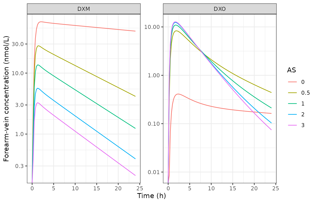
# At 3 h (around the DXM peak) higher AS gives lower DXM and (up to AS 1) more
# DXO, exactly the monotone CYP2D6 effect the paper reports.
peak <- prof[abs(prof$time - 3) < 1e-6, ]
peak <- peak[order(as.numeric(as.character(peak$AS))), ]
stopifnot(
  all(diff(peak$DXM) < 0), # DXM strictly decreases with AS
  peak$DXO[peak$AS == "1"] > peak$DXO[peak$AS == "0"]
)
UCMR and metabolic phenotype (Figure 9, Figure 11)
The UCMR is the model’s clinical readout. The paper assigns phenotypes with the cutoffs PM: UCMR >= 0.3; IM: 0.03 <= UCMR < 0.3; EM: 0.0003 <= UCMR < 0.03; UM: UCMR < 0.0003 (Section 2.4). The typical-value UCMR at 8 h falls neatly into the expected phenotype band for each activity score.
classify <- function(u) {
  ifelse(u >= 0.3, "PM",
    ifelse(u >= 0.03, "IM",
      ifelse(u >= 0.0003, "EM", "UM")
    )
  )
}
ucmr8 <- sapply(c(0, 0.25, 0.5, 1, 1.25, 1.5, 2, 3), function(as) {
  s <- rxode2::rxSolve(mod_typ, oral_events(as, tmax = 480, by = 30),
    returnType = "data.frame"
  )
  s$UCMR[s$time == 480]
})
#> ℹ omega/sigma items treated as zero: 'etalvmax2d6', 'etalkm2d6', 'etalvmax3a4', 'etalkm3a4'
#> ℹ omega/sigma items treated as zero: 'etalvmax2d6', 'etalkm2d6', 'etalvmax3a4', 'etalkm3a4'
#> ℹ omega/sigma items treated as zero: 'etalvmax2d6', 'etalkm2d6', 'etalvmax3a4', 'etalkm3a4'
#> ℹ omega/sigma items treated as zero: 'etalvmax2d6', 'etalkm2d6', 'etalvmax3a4', 'etalkm3a4'
#> ℹ omega/sigma items treated as zero: 'etalvmax2d6', 'etalkm2d6', 'etalvmax3a4', 'etalkm3a4'
#> ℹ omega/sigma items treated as zero: 'etalvmax2d6', 'etalkm2d6', 'etalvmax3a4', 'etalkm3a4'
#> ℹ omega/sigma items treated as zero: 'etalvmax2d6', 'etalkm2d6', 'etalvmax3a4', 'etalkm3a4'
#> ℹ omega/sigma items treated as zero: 'etalvmax2d6', 'etalkm2d6', 'etalvmax3a4', 'etalkm3a4'
as_vals <- c(0, 0.25, 0.5, 1, 1.25, 1.5, 2, 3)
tab <- data.frame(AS = as_vals, UCMR_8h = round(ucmr8, 4), phenotype = classify(ucmr8))
tab
#>     AS UCMR_8h phenotype
#> 1 0.00  1.3986        PM
#> 2 0.25  0.0703        IM
#> 3 0.50  0.0275        EM
#> 4 1.00  0.0103        EM
#> 5 1.25  0.0075        EM
#> 6 1.50  0.0058        EM
#> 7 2.00  0.0038        EM
#> 8 3.00  0.0021        EM

# AS 0 is a poor metabolizer; every functional activity score is an extensive
# metabolizer, and UCMR decreases monotonically with activity score -- the
# paper's genotype-phenotype association (Figure 11).
stopifnot(
  tab$phenotype[tab$AS == 0] == "PM",
  all(tab$phenotype[tab$AS >= 1] == "EM"),
  all(diff(ucmr8) < 0)
)
Virtual cohort: UCMR distribution (Figure 11)
The between-subject variability in the hepatic CYP2D6 and CYP3A4 Km and Vmax produces a distribution of UCMR at each activity score. Simulating a cohort at three activity scores reproduces the overlapping-but-ordered UCMR distributions of Figure 11: PM (AS 0) sits well above the EM range, while AS 1 and AS 2 sit within it and overlap.
rxode2::rxSetSeed(1234)
n_sub <- 120
cohort <- lapply(c(0, 1, 2), function(as) {
  ev <- rxode2::et(amt = 30, cmt = "depot") |>
    rxode2::et(480) |>
    rxode2::et(id = seq_len(n_sub)) |>
    as.data.frame() |>
    dplyr::mutate(WT = 75, CYP2D6 = as)
  s <- rxode2::rxSolve(mod, ev, returnType = "data.frame")
  s <- s[s$time == 480, ]
  data.frame(AS = factor(as), UCMR = s$UCMR)
})
cohort <- do.call(rbind, cohort)

ggplot(cohort, aes(AS, UCMR)) +
  geom_boxplot(outlier.size = 0.6) +
  scale_y_log10() +
  geom_hline(yintercept = c(0.3, 0.03, 0.0003), linetype = "dashed") +
  labs(
    x = "CYP2D6 activity score", y = "UCMR at 8 h (log scale)",
    caption = "Dashed lines: PM/IM, IM/EM, EM/UM cutoffs"
  ) +
  theme_bw()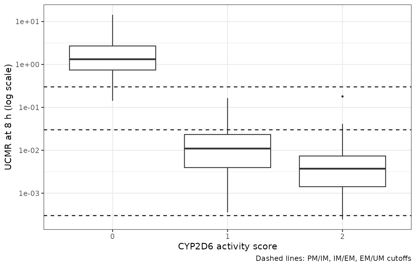
Non-compartmental analysis
The paper validates against concentration-time profiles and urinary ratios rather than a table of non-compartmental parameters, so there is no published NCA table to compare against. We still run PKNCA on the simulated 30 mg oral DXM profile as a structural sanity check: the extensive metabolizers (AS 1, 2) must show a much lower DXM exposure and shorter half-life than the poor metabolizer (AS 0).
conc_data <- lapply(c(0, 1, 2), function(as) {
  s <- rxode2::rxSolve(mod_typ, oral_events(as, tmax = 2880, by = 30),
    returnType = "data.frame"
  )
  data.frame(id = 1, treatment = paste0("AS", as), time = s$time / 60, Cc = s$Cc)
})
conc_data <- do.call(rbind, conc_data)
conc_data <- dplyr::filter(conc_data, !is.na(Cc))

dose_data <- data.frame(
  id = 1, treatment = paste0("AS", c(0, 1, 2)), time = 0, dose_mg = 30
)

o_conc <- PKNCA::PKNCAconc(conc_data, Cc ~ time | treatment + id)
o_dose <- PKNCA::PKNCAdose(dose_data, dose_mg ~ time | treatment + id)
nca_res <- suppressMessages(PKNCA::pk.nca(PKNCA::PKNCAdata(o_conc, o_dose)))

nca_wide <- nca_res$result |>
  dplyr::filter(PPTESTCD %in% c("cmax", "tmax", "auclast", "half.life")) |>
  dplyr::select(treatment, PPTESTCD, PPORRES) |>
  tidyr::pivot_wider(names_from = PPTESTCD, values_from = PPORRES)
nca_wide |>
  dplyr::rename(
    "Treatment" = treatment, "Cmax (nmol/L)" = cmax, "Tmax (h)" = tmax,
    "AUClast (nmol*h/L)" = auclast, "t1/2 (h)" = half.life
  ) |>
knitr::kable(digits = 3)| Treatment | AUClast (nmol*h/L) | Cmax (nmol/L) | Tmax (h) | t1/2 (h) |
|---|---|---|---|---|
| AS0 | 1362.966 | 69.395 | 2.0 | 45.214 |
| AS1 | 125.502 | 13.554 | 1.5 | 6.644 |
| AS2 | 48.289 | 5.585 | 1.5 | 5.974 |
Mass balance
At the end of the simulation the drug-related mass should be conserved: the dose equals the amount recovered in urine (as DXM, DXO and DXO-Glu) plus feces plus the small amount remaining in the body and the DXM lost to the CYP3A4 N-demethylation “annihilation” sink. We check the recoverable fractions grow monotonically and stay below the dose.
s <- rxode2::rxSolve(mod_typ, oral_events(1, tmax = 4320, by = 60),
  returnType = "data.frame"
)
#> ℹ omega/sigma items treated as zero: 'etalvmax2d6', 'etalkm2d6', 'etalvmax3a4', 'etalkm3a4'
last <- s[nrow(s), ]
dose_mmol <- 30 / 271.404
recovered <- last$Aurine_dxm + last$Aurine_dxo + last$Aurine_dxoglu + last$feces
# Recovered mass is positive, below the dose, and feces is the 45% unabsorbed.
stopifnot(
  recovered > 0,
  recovered < dose_mmol,
  abs(last$feces / dose_mmol - 0.45) < 0.01
)
round(c(
  dose_mmol = dose_mmol, feces = last$feces,
  urine_dxm = last$Aurine_dxm, urine_dxo = last$Aurine_dxo,
  urine_dxoglu = last$Aurine_dxoglu
), 5)
#>    dose_mmol        feces    urine_dxm    urine_dxo urine_dxoglu
#>      0.11054      0.04974      0.00053      0.00171      0.03470
Assumptions and deviations / Errata
Rate laws and physiological constants from the model archive. The paper prints its parameter values (Table 2) but not its rate laws or the full set of fractional blood-pool volumes. These were taken from the model archive the paper names as the version used (Section 2.2): Grzegorzewski & Koenig, dextromethorphan-model v0.9.5, doi:10.5281/zenodo.7025683. The port is verified to reproduce that archive exactly (see “Reproducing the deposited SBML model”).
Dissolution rate unit. Table 2 and the archive store
Ka_dis_dxmas 0.0217 with unit “1/hr”. Taken literally, a 0.0217/hr dissolution gives a dextromethorphan Tmax beyond 24 h, which contradicts the 1–2 h Tmax of every oral panel in Figures 3 and 4. Interpreting the stored value as 0.0217 /min (= 1.304 /hr) reproduces those figures, so the model uses 1.304 /hr. This is the only value changed from the archive; all other parameters are used as deposited.Forearm venous mixing. The archive’s forearm-outflow reaction lists both the forearm plasma and the arterial blood as stoichiometry-1 reactants, so each loses the full summed flux of that reaction (not only its own term). The port reproduces this exactly; it is what makes the forearm-vein concentration – the paper’s sampling site – match the archive.
Forearm volume does not scale with body weight. In the archive the forearm compartment is fixed at 1 L (its fractional volume enters only the rest-of-body balance). The port keeps this; only the forearm volumes are body-weight-independent.
Between-subject variability digitised from Figure 2. The paper models CYP2D6 and CYP3A4 variability as correlated bivariate log-normal distributions of Km and Vmax fitted to human liver microsome data, but reports no numeric dispersion or correlation. The variances and correlations in the model were digitised by the maintainers from Figure 2: the CYP3A4 values from the normalised joint distribution in panel 2A, and the CYP2D6 within-activity-score values from the per-score panels of 2B. They reproduce the shape and spread of Figure 2 and the UCMR dispersion of Figure 11 but are approximate; treat them as the published figure, not as tabulated estimates. The variability is applied to the hepatic enzymes only (the Figure 2 source data are hepatic microsomes); the gut-wall CYP3A4 first-pass uses the deterministic Table 2 value.
CYP2D6 activity score as a covariate. The archive can take a diplotype as two allele indices and map them to an activity score through a 170-branch lookup (Supplementary Table S1). The port exposes the resulting activity score directly as the continuous covariate
CYP2D6(0–4); supply the activity score for the diplotype of interest.AS = 0removes the CYP2D6 pathway.No residual-error model. The paper’s variability is entirely in the enzyme Km/Vmax distributions; there is no separate residual-error term, so
propSdis fixed at zero and the cohort spread comes from the enzyme IIV.Quinidine inhibition omitted. The archive carries an (inactive by default) competitive quinidine-inhibition term on the hepatic CYP2D6 reaction for its drug-drug-interaction scenarios. This base model simulates no quinidine, so the term is omitted; the model is not a DDI model.