Model and source
- Citation: Yin W, Facius A, Wagner T, Tsai M, Asgharnejad M, Lahu G, Vakilynejad M. Population pharmacokinetics, enzyme occupancy, and 24S-hydroxycholesterol modeling of soticlestat, a novel cholesterol 24-hydroxylase inhibitor, in healthy adults. Clin Transl Sci. 2023;16(7):1149-1162. doi:10.1111/cts.13517. Structural equations from Appendix S1 (NONMEM control streams, three sections) and Appendix S2 (population PK differential equations); all shipped values from Table 2. The CH24H enzyme-occupancy sub-model estimated here is carried forward FIXED into the patient model of Yin W, Facius A, Asgharnejad M, Lahu G, Vakilynejad M. Population pharmacokinetics, enzyme occupancy, and pharmacodynamic modeling of soticlestat in patients with developmental and epileptic encephalopathies. Clin Transl Sci. 2024;17(3):e13722. doi:10.1111/cts.13722; see modellib(‘Yin_2024_soticlestat’).
- Description: Joint population PK / CH24H enzyme-occupancy (EO) / 24S-hydroxycholesterol (24HC) pharmacodynamic model for soticlestat (TAK-935), a first-in-class selective inhibitor of cholesterol 24-hydroxylase (CH24H / CYP46A1), in healthy adults (Yin 2023). Two-compartment PK with first-order absorption fed by an explicit two-compartment transit chain that is the dosing route for the tablet formulation, the oral solution dosing directly into the absorption depot; empirical dose-nonlinearity power terms on CL/F, Q/F and Vp/F; a plasma-to-brain effect compartment whose concentration drives both a sigmoid Emax brain CH24H enzyme-occupancy read-out and a semimechanistic sigmoid Imax inhibitory indirect-response turnover model for plasma 24HC. Weight-based allometry on CL/F, Vc/F, Q/F and Vp/F (reference 70 kg) was added by the authors after estimation to support the paediatric dosing simulations.
- Article: https://doi.org/10.1111/cts.13517
- Supplement: Appendix S1 (three NONMEM control streams: popPK, PK/EO, PK/24HC), Appendix S2 (population PK differential equations), Tables S1-S4 and Figures S1-S3, all in the Supporting Information of https://doi.org/10.1111/cts.13517
Soticlestat (TAK-935) is a first-in-class selective inhibitor of cholesterol 24-hydroxylase (CH24H / CYP46A1), the brain-specific enzyme that catabolizes cholesterol to 24S-hydroxycholesterol (24HC). It is in phase III development for Dravet syndrome and Lennox-Gastaut syndrome. This paper develops a single joint model over three linked layers, each fitted in sequence:
- a population PK model for plasma soticlestat;
- a PK/EO model linking an effect-site concentration
to brain CH24H enzyme occupancy measured by
[18F]MNI-792PET; and - a PK/PD model in which that same effect-site concentration inhibits the production of plasma 24HC through an indirect-response turnover model.
Because the three layers share one effect compartment and one PK
backbone, they are shipped as a single coupled model file with three
observation endpoints (Cc, occ,
hc24) rather than three separate models.
The immediate successor analysis, which refits this structure in
patients with developmental and epileptic encephalopathies and carries
the enzyme-occupancy sub-model forward fixed from this paper,
is available as modellib("Yin_2024_soticlestat").
Population
The model was built from four phase I studies in healthy adults (Table 1), enrolling 108 participants in total (Table S1):
| Study | Design | n | Dosing |
|---|---|---|---|
| NCT02201056 | single rising dose | 48 | 15, 50, 200, 600, 900, 1350 mg single dose, oral solution |
| NCT02539134 | multiple rising dose | 40 | 100, 300, 400, 600 mg q.d. and 300 mg b.i.d. for 10-14 days, oral solution |
| NCT02497235 | open-label PET occupancy | 11 | 50, 100, 200, 300, 600 mg single dose, oral solution |
| NCT02906813 | relative bioavailability / food effect | 9 | 300 mg single dose as 3 x 100 mg tablets (fed or fasted) or oral solution |
Participants had a mean (SD) age of 34.7 (9.6) years and a mean (SD) body mass index of 25.6 (2.9) kg/m^2; 74/108 (69%) were men, and 78 (72%) were White, 28 (26%) Black or African American and 2 (2%) multiracial (Table S1).
The three layers were fitted to three overlapping analysis sets: the
population PK model used 1727 soticlestat concentrations from 104
individuals, the PK/EO model 20 brain occupancy observations from 11
individuals, and the PK/PD model 2270 plasma 24HC concentrations from 99
individuals. No data were excluded or imputed. All dosing was oral and
no intravenous data were available, so absolute bioavailability could
not be estimated and every clearance and volume is an apparent
(/F) parameter.
The same information is available programmatically via the model’s
population metadata
(readModelDb("Yin_2023_soticlestat")()$population).
Source trace
The per-parameter origin is recorded as an in-file comment next to
each ini() entry in
inst/modeldb/specificDrugs/Yin_2023_soticlestat.R. The
table below collects them in one place. Every shipped value comes from
Table 2, the “Original / Estimate” column; the Appendix
S1 $THETA / $OMEGA blocks hold
initial estimates (CL 220, Vc 60, ka 2.0) and are used only for
structure and for the FIX flags.
| Equation / parameter | Value | Source location |
|---|---|---|
Structure:
transit1 -> transit2 -> depot -> central <-> peripheral1
|
– | Appendix S2 (differential equations) and Appendix S1 popPK
$DES
|
Tablet doses into transit1; solution into
depot
|
– | Appendix S2 caption: “The transit compartment 1 is the dosing
compartment for the tablet formulation”;
COMP=(DEPOT,DEFDOSE)
|
lka (ka) |
2.13 1/h | Table 2, Absorption rate (ka), TV |
lktr (ktr) |
2.47 1/h | Table 2, Transit rate for tablets (ktr), TV |
lcl (CL/F at 300 mg) |
204 L/h | Table 2, Oral clearance (CL/F), TV |
lvc (Vc/F) |
65.5 L | Table 2, Volume of distribution of the central compartment (Vc/F), TV |
lq (Q/F at 300 mg) |
52.6 L/h | Table 2, Intercompartmental apparent clearance (Q/F), TV |
lvp (Vp/F at 300 mg) |
356 L | Table 2, Apparent volume of distribution for the peripheral compartment (Vp/F), TV |
e_dose_cl |
-0.278 | Table 2, CL/F Dose effect (exponent) |
e_dose_q |
-0.554 | Table 2, Q/F Dose effect (exponent) |
e_dose_vp |
-0.684 | Table 2, Vp/F Dose effect (exponent) |
e_wt_cl |
0.75 (fixed) | Paper “PopPK model”:
CL/F = (Dose/300)^-0.278 * (Weight/70)^0.75 * 204 L/h
|
e_wt_vc |
1 (fixed) | Paper “PopPK model”: Vc/F = 65.5 * (Weight/70)^-1 L –
sign corrected, see Errata |
e_wt_q, e_wt_vp
|
0.75, 1 (fixed) | Not printed by the paper – standard allometric exponents assumed, see Errata |
etalcl .. etalktr
|
0.353, 0.562, 0.418, 0.616, 0.981 (SD) | Table 2 BSV rows, squared into variances – see “BSV scale” below |
etalka |
0 (fixed) | Table 2, ka BSV “0 Fixed”; popPK $OMEGA 5
0 FIX
|
propSd |
0.454 | Table 2, Residual variability Proportional (%) 45.4 |
addSd |
0.001 (fixed) | Table 2, Residual variability Additive (ng/mL), Fixed |
Effect site: d/dt(effect) = kEO * (Cc - effect)
|
– | Paper “PK/EO model” equation;
DADT(6) = KEO*(A(2)/S2-A(6))
|
lke0 (kEO) |
0.255 1/h | Table 2, Delay rate (kEO), TV |
lemax (Emax) |
100 % (fixed) | Table 2, Maximum EO (Emax), TV, Fixed; PK/EO $THETA 4
(100) FIX
|
lec50 (EC50) |
5.86 ng/mL | Table 2, EO EC50, TV |
lhill_eo (gamma) |
0.769 | Table 2, EO Shape parameter (gamma), TV |
etalec50 |
0.692 (SD) | Table 2, EO EC50 BSV |
addSd_occ |
2.88 % occupancy | Table 2, EO Residual variability Additive; Proportional “0 Fixed” |
occ = Emax * ce^g / (EC50^g + ce^g) |
– | Paper “PK/EO model” equation; PK/EO $ERROR
|
lrbase (BL24HC) |
45.9 ng/mL | Table 2, Baseline 24HC (BL24HC), TV |
lkout (kout) |
0.0182 1/h | Table 2, 24HC degradation rate (kout), TV |
limax (Imax) |
78.2 % | Table 2, Maximum 24HC inhibition (Imax), TV |
lic50 (IC50) |
5.21 ng/mL | Table 2, 24HC IC50, TV |
lhill_hc24 |
1 (fixed) | PK/24HC $THETA 11 IGAM 1 FIX;
$DES writes the sigmoid with no exponent |
etalrbase, etalkout
|
0.474, 0.631 (SD) | Table 2, BL24HC and kout BSV rows |
propSd_hc24 |
0.001 (fixed) | Table 2, 24HC Residual variability Proportional, Fixed |
addSd_hc24 |
3.4 ng/mL | Table 2, 24HC Residual variability Additive |
kin = BL24HC * kout, hc24(0) = BL24HC
|
– | PK/24HC $PK: A_0(7) = BL,
KIN = BL*KOUT
|
d/dt(hc24) = kin*(1-Imax/100*ce/(ce+IC50)) - kout*hc24 |
– | Paper “PK/PD model” equation; $DES
EFF = 1 - IMAX*A(6)/(A(6)+IC50)
|
BSV scale: Table 2 reports standard deviations, not variances
Table 2’s between-subject-variability rows need care, because the “Estimate” column and the “95% CI” column are on different scales. Two independent lines of evidence establish that the estimate is an omega standard deviation while the CI is on the omega variance, so the model file ships the squares: an internal-consistency check on the CIs, and a match against the CVs the paper states in prose.
bsv <- tibble::tribble(
  ~parameter,  ~printed, ~ci_low, ~ci_high,
  "CL/F",         0.353,   0.075,   0.177,
  "Vc/F",         0.562,   0.157,   0.526,
  "Q/F",          0.418,  0.0548,   0.319,
  "Vp/F",         0.616,   0.187,   0.656,
  "ktr",          0.981,   0.458,    1.56,
  "EO EC50",      0.692,   0.113,   0.661,
  "BL24HC",       0.474,   0.199,   0.245,
  "kout",         0.631,   0.178,   0.548
) |>
  mutate(
    printed_in_ci = printed >= ci_low & printed <= ci_high,
    square        = printed^2,
    square_in_ci  = square >= ci_low & square <= ci_high
  )

bsv |>
  rename(
    "Parameter" = parameter, "Table 2 estimate" = printed,
    "CI low" = ci_low, "CI high" = ci_high,
    "Estimate in own CI?" = printed_in_ci,
    "Estimate^2" = square, "Estimate^2 in CI?" = square_in_ci
  ) |>
knitr::kable(digits = 4, caption = "Table 2 BSV rows: the square of the printed estimate lies inside the row's own CI in all 8 rows, while the printed estimate itself lies outside in 6 of the 8.")| Parameter | Table 2 estimate | CI low | CI high | Estimate in own CI? | Estimate^2 | Estimate^2 in CI? |
|---|---|---|---|---|---|---|
| CL/F | 0.353 | 0.0750 | 0.177 | FALSE | 0.1246 | TRUE |
| Vc/F | 0.562 | 0.1570 | 0.526 | FALSE | 0.3158 | TRUE |
| Q/F | 0.418 | 0.0548 | 0.319 | FALSE | 0.1747 | TRUE |
| Vp/F | 0.616 | 0.1870 | 0.656 | TRUE | 0.3795 | TRUE |
| ktr | 0.981 | 0.4580 | 1.560 | TRUE | 0.9624 | TRUE |
| EO EC50 | 0.692 | 0.1130 | 0.661 | FALSE | 0.4789 | TRUE |
| BL24HC | 0.474 | 0.1990 | 0.245 | FALSE | 0.2247 | TRUE |
| kout | 0.631 | 0.1780 | 0.548 | FALSE | 0.3982 | TRUE |
# Proof 1: the square is inside the row's own CI in EVERY row (8/8), whereas
# the printed estimate itself is outside its own CI in 6 of the 8 rows. Reading
# the printed number as a variance is therefore impossible for those 6 rows.
# The remaining 2 rows (Vp/F and ktr) have CIs wide enough to contain both
# readings, so they are simply uninformative rather than contradictory -- the
# counts are asserted exactly so that a future transcription slip in any row
# fails this gate.
stopifnot(
  all(bsv$square_in_ci),
  sum(!bsv$printed_in_ci) == 6L,
  # the two uninformative rows are exactly the ones named above
  identical(sort(bsv$parameter[bsv$printed_in_ci]), c("ktr", "Vp/F"))
)

# Proof 2: reading the printed numbers as SDs reproduces the prose CVs.
# Paper: CL "a coefficient of variation (CV) of 36%", Vc "a CV of 61%".
cv <- function(omega_sq) 100 * sqrt(exp(omega_sq) - 1)
cv_as_sd  <- c(CL = cv(0.353^2), Vc = cv(0.562^2))
cv_as_var <- c(CL = cv(0.353),   Vc = cv(0.562))
print(round(rbind(`read as SD` = cv_as_sd, `read as variance` = cv_as_var), 1))
#>                    CL   Vc
#> read as SD       36.4 60.9
#> read as variance 65.1 86.8
stopifnot(
  abs(cv_as_sd[["CL"]] - 36) < 1,
  abs(cv_as_sd[["Vc"]] - 61) < 1,
  # the variance reading misses both published CVs by a wide margin
  abs(cv_as_var[["CL"]] - 36) > 20,
  abs(cv_as_var[["Vc"]] - 61) > 20
)
Dimensional analysis
The 24HC layer is an endogenous turnover model, so the units of every ODE term are checked explicitly rather than assumed.
| Term | Units | Notes |
|---|---|---|
transit1, transit2, depot,
central, peripheral1
|
mg | amounts; dose is in mg |
ka, ktr, kout,
ke0
|
1/h | first-order rate constants |
cl, q
|
L/h | apparent (/F) clearances |
vc, vp
|
L | apparent (/F) volumes |
Cc = 1000 * central / vc |
ng/mL |
mg/L * 1000 = ng/mL; reproduces NONMEM
S2 = Vc/1000
|
effect, ce
|
ng/mL | a concentration, not an amount:
d/dt(effect) = ke0 * (Cc - effect)
|
ec50, ic50
|
ng/mL | matched to ce
|
hill_eo, hill_hc24
|
unitless | exponents |
emax, imax
|
% |
occ is a percentage; imax is divided by
100 to give a fraction |
drugEff |
unitless | fraction in [0, 1)
|
hc24, rbase
|
ng/mL | plasma 24HC concentration |
kin = rbase * kout |
ng/mL/h | matches kout * hc24 on the other side of the
balance |
d/dt(hc24) |
ng/mL/h | consistent |
The only non-obvious conversion is the factor of 1000 in
Cc, which carries mg/L into ng/mL and reproduces the NONMEM
scale factor S2 = Vc/1000 exactly. The effect compartment
is unusual in holding a concentration rather than an amount; that is
what the published ODE specifies.
mod <- rxode2::rxode(readModelDb("Yin_2023_soticlestat"))
#> ℹ parameter labels from comments will be replaced by 'label()'

# Helper: this model has three `~` endpoints, so every observation row needs a
# `dvid`. Setting dvid = 1L on all observation rows returns every endpoint
# column (Cc, occ, hc24) at each observation time.
withDvid <- function(ev) {
  ev <- as.data.frame(ev)
  ev$dvid <- ifelse(ev$evid == 0, 1L, NA_integer_)
  ev
}
# Typical-value (population) version, for reproducing published typical curves.
modTv <- rxode2::zeroRe(mod)
Structural verification
Three structural properties are asserted before any figure is reproduced, because each one is a distinct way the translation could be silently wrong.
The disposition is genuinely two-compartment
A two-compartment model written with micro-constants can be silently
collapsed to one compartment by rxSolve’s automatic
linCmt() conversion. The check below confirms the
peripheral compartment actually loads and that the observed terminal
slope equals the analytic beta eigenvalue of the two-compartment
system.
rxode2::rxSetSeed(1024)
evSingle <- withDvid(
  rxode2::et(amt = 300, cmt = "transit1") |>
    rxode2::et(seq(0, 96, by = 0.05), cmt = "central")
)
sTab <- as.data.frame(rxode2::rxSolve(modTv, evSingle, params = c(DOSE = 300, WT = 70)))
#> ℹ omega/sigma items treated as zero: 'etalcl', 'etalvc', 'etalq', 'etalvp', 'etalktr', 'etalka', 'etalec50', 'etalrbase', 'etalkout'

p <- sTab[1, ]
k10 <- p$cl / p$vc
k12 <- p$q / p$vc
k21 <- p$q / p$vp
betaAnalytic <- 0.5 * ((k10 + k12 + k21) - sqrt((k10 + k12 + k21)^2 - 4 * k10 * k21))

# Keep Cc >= 1e-6 * Cmax: below that the ODE integrator has no relative accuracy left.
tail96 <- subset(sTab, time >= 48 & time <= 96 & Cc >= 1e-6 * max(Cc))
betaObserved <- -stats::coef(stats::lm(log(tail96$Cc) ~ tail96$time))[[2]]

cat(sprintf("peripheral1 peak amount     : %.2f mg\n", max(sTab$peripheral1)))
#> peripheral1 peak amount     : 48.36 mg
cat(sprintf("analytic beta               : %.6f 1/h (t1/2 %.2f h)\n",
            betaAnalytic, log(2) / betaAnalytic))
#> analytic beta               : 0.116537 1/h (t1/2 5.95 h)
cat(sprintf("observed terminal slope     : %.6f 1/h (t1/2 %.2f h)\n",
            betaObserved, log(2) / betaObserved))
#> observed terminal slope     : 0.116537 1/h (t1/2 5.95 h)

stopifnot(
  # the peripheral compartment must actually receive drug
  max(sTab$peripheral1) > 1,
  # and the terminal phase must be the two-compartment beta, not cl/vc
  abs(betaObserved / betaAnalytic - 1) < 0.01,
  # a one-compartment collapse would give the much faster kel = cl/vc
  abs(betaObserved / k10 - 1) > 0.5
)
The transit chain delays absorption without losing dose
The tablet route runs through two transit compartments; the oral
solution doses straight into depot. Both must deliver the
same amount of drug – a transit chain that lost dose would silently bias
every tablet-based simulation.
evSol <- withDvid(
  rxode2::et(amt = 300, cmt = "depot") |>
    rxode2::et(seq(0, 96, by = 0.05), cmt = "central")
)
sSol <- as.data.frame(rxode2::rxSolve(modTv, evSol, params = c(DOSE = 300, WT = 70)))
#> ℹ omega/sigma items treated as zero: 'etalcl', 'etalvc', 'etalq', 'etalvp', 'etalktr', 'etalka', 'etalec50', 'etalrbase', 'etalkout'

trapz <- function(x, y) sum(diff(x) * (utils::head(y, -1) + utils::tail(y, -1)) / 2)
aucTab <- trapz(sTab$time, sTab$Cc)
aucSol <- trapz(sSol$time, sSol$Cc)

routes <- tibble::tibble(
  Route = c("Oral solution (doses into depot)", "Tablet (doses into transit1)"),
  Tmax = c(sSol$time[which.max(sSol$Cc)], sTab$time[which.max(sTab$Cc)]),
  Cmax = c(max(sSol$Cc), max(sTab$Cc)),
  AUC = c(aucSol, aucTab)
)
routes |>
  rename("Tmax (h)" = Tmax, "Cmax (ng/mL)" = Cmax, "AUC0-96 (ng*h/mL)" = AUC) |>
knitr::kable(digits = 2, caption = "Tablet vs oral solution after a 300 mg dose (typical values). The transit chain delays and blunts the peak but conserves AUC.")| Route | Tmax (h) | Cmax (ng/mL) | AUC0-96 (ng*h/mL) |
|---|---|---|---|
| Oral solution (doses into depot) | 0.35 | 1207.90 | 1468.55 |
| Tablet (doses into transit1) | 1.15 | 686.48 | 1470.58 |
Setting WT = 70 recovers the estimated adult model
The weight terms were added by the authors after estimation, to support the paediatric simulations. At the 70 kg reference every allometric factor must collapse to exactly 1.
pRef <- sTab[1, ]
stopifnot(
  # at WT = 70 and DOSE = 300 every covariate factor is 1, so the individual
  # parameters must equal the Table 2 typical values exactly
  abs(pRef$cl - 204) < 1e-6,
  abs(pRef$vc - 65.5) < 1e-6,
  abs(pRef$q - 52.6) < 1e-6,
  abs(pRef$vp - 356) < 1e-6,
  abs(pRef$ka - 2.13) < 1e-6,
  abs(pRef$ktr - 2.47) < 1e-6
)
cat("WT = 70, DOSE = 300 reproduces every Table 2 typical value exactly.\n")
#> WT = 70, DOSE = 300 reproduces every Table 2 typical value exactly.
Endogenous validation of the 24HC layer
Plasma 24HC is an endogenous biomarker described by an indirect-response turnover model. NCA is not a meaningful check for it, so the four endogenous-model validations are used instead. (The soticlestat PK layer does get the standard PKNCA treatment, further below.)
1. Steady-state hold
With no drug present the pool must sit at its own baseline indefinitely.
evNone <- withDvid(rxode2::et(seq(0, 60 * 24, by = 6), cmt = "central"))
sNone <- as.data.frame(rxode2::rxSolve(modTv, evNone, params = c(DOSE = 300, WT = 70)))
#> ℹ omega/sigma items treated as zero: 'etalcl', 'etalvc', 'etalq', 'etalvp', 'etalktr', 'etalka', 'etalec50', 'etalrbase', 'etalkout'

cat(sprintf("hc24 over 60 drug-free days: [%.10f, %.10f], baseline %.4f\n",
            min(sNone$hc24), max(sNone$hc24), sNone$rbase[1]))
#> hc24 over 60 drug-free days: [45.9000000000, 45.9000000000], baseline 45.9000
stopifnot(
  # the drug-free system is at steady state by construction (kin = rbase*kout)
  max(abs(sNone$hc24 - sNone$rbase[1])) < 1e-8,
  # and with no drug the occupancy read-out must be exactly zero
  max(sNone$occ) < 1e-12
)
2. Mass-balance / flux check
At baseline, production and elimination must cancel exactly.
p0 <- sNone[1, ]
production <- p0$kin
elimination <- p0$kout * p0$hc24
cat(sprintf("kin = BL24HC * kout = %.4f * %.6f = %.8f ng/mL/h\n",
            p0$rbase, p0$kout, production))
#> kin = BL24HC * kout = 45.9000 * 0.018200 = 0.83538000 ng/mL/h
cat(sprintf("kout * hc24(0)      = %.6f * %.4f = %.8f ng/mL/h\n",
            p0$kout, p0$hc24, elimination))
#> kout * hc24(0)      = 0.018200 * 45.9000 = 0.83538000 ng/mL/h
cat(sprintf("net flux            = %.3e ng/mL/h\n", production - elimination))
#> net flux            = 0.000e+00 ng/mL/h
stopifnot(abs(production - elimination) < 1e-12)
3. Perturbation recovery
The model sets its own initial condition
(hc24(0) <- rbase), so passing inits= does
not perturb the pool – a naive perturbation test here
would silently assert nothing. The perturbation is therefore applied the
way the drug applies it: dose for 21 days to drive 24HC down, then
withdraw and confirm the pool returns to its own baseline over the 7-day
washout, which is exactly the experiment plotted in Figure 4c.
evWash <- withDvid(
  rxode2::et(amt = 300, cmt = "transit1", ii = 12, until = 21 * 24 - 12) |>
    rxode2::et(seq(0, 28 * 24, by = 1), cmt = "central")
)
sWash <- as.data.frame(rxode2::rxSolve(modTv, evWash, params = c(DOSE = 300, WT = 70)))
#> ℹ omega/sigma items treated as zero: 'etalcl', 'etalvc', 'etalq', 'etalvp', 'etalktr', 'etalka', 'etalec50', 'etalrbase', 'etalkout'

nadir <- min(sWash$hc24)
endOfWashout <- sWash$hc24[which.max(sWash$time)]
baseline <- sWash$rbase[1]
cat(sprintf("baseline %.2f -> nadir %.2f (%.1f%% of baseline) -> day 28 %.2f (%.1f%% of baseline)\n",
            baseline, nadir, 100 * nadir / baseline,
            endOfWashout, 100 * endOfWashout / baseline))
#> baseline 45.90 -> nadir 11.87 (25.9% of baseline) -> day 28 43.66 (95.1% of baseline)

stopifnot(
  # the drug must genuinely displace the pool (this is what makes the test real)
  nadir < 0.4 * baseline,
  # and it must come back after 7 days of washout
  endOfWashout > 0.9 * baseline,
  # monotone recovery from the nadir to the end of washout
  endOfWashout > nadir
)
ggplot(sWash, aes(time / 24, hc24)) +
  geom_hline(yintercept = baseline, linetype = "dashed", colour = "grey40") +
  geom_line(linewidth = 0.7) +
  geom_vline(xintercept = 21, linetype = "dotted") +
  labs(x = "Time (days)", y = "Plasma 24HC (ng/mL)") +
  theme_bw()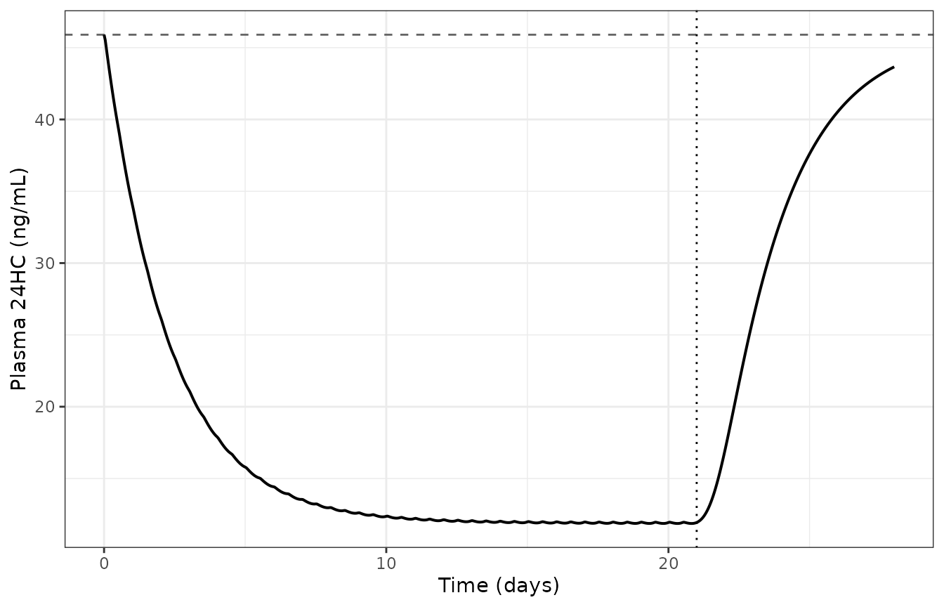
Perturbation-recovery of the plasma 24HC pool: 21 days of soticlestat 300 mg b.i.d. followed by a 7-day washout (typical values). Reproduces the shape of Figure 4c of Yin 2023.
Replication of the published simulations
Figure 4: 300 mg b.i.d. versus 600 mg q.d.
The paper simulates 21 days of dosing followed by a 7-day washout for a typical 70 kg adult and reports that b.i.d. dosing spends a greater proportion of time above the 65% target CH24H occupancy, with lower fluctuation, than the equivalent total daily dose given once daily (Figure 4).
rxode2::rxSetSeed(20230717)
regimens <- tibble::tribble(
  ~label,            ~dose, ~ii,
  "300 mg b.i.d.",     300,  12,
  "600 mg q.d.",       600,  24
)

simRegimen <- function(dose, ii, label, nSub = 1L, seed = NULL) {
  if (!is.null(seed)) rxode2::rxSetSeed(seed)
  ev <- withDvid(
    rxode2::et(amt = dose, cmt = "transit1", ii = ii, until = 21 * 24 - ii) |>
      rxode2::et(seq(0, 28 * 24, by = 1), cmt = "central")
  )
  m <- if (nSub > 1L) mod else modTv
  s <- as.data.frame(rxode2::rxSolve(m, ev, params = c(DOSE = dose, WT = 70),
                                     nSub = nSub))
  s$label <- label
  s
}

fig4 <- bind_rows(Map(function(d, i, l) simRegimen(d, i, l),
                      regimens$dose, regimens$ii, regimens$label))
#> ℹ omega/sigma items treated as zero: 'etalcl', 'etalvc', 'etalq', 'etalvp', 'etalktr', 'etalka', 'etalec50', 'etalrbase', 'etalkout'
#> ℹ omega/sigma items treated as zero: 'etalcl', 'etalvc', 'etalq', 'etalvp', 'etalktr', 'etalka', 'etalec50', 'etalrbase', 'etalkout'

fig4long <- fig4 |>
  select(time, label, Cc, occ, hc24Chg) |>
  pivot_longer(c(Cc, occ, hc24Chg), names_to = "endpoint", values_to = "value") |>
  mutate(endpoint = factor(
    endpoint, levels = c("Cc", "occ", "hc24Chg"),
    labels = c("Soticlestat (ng/mL)", "CH24H occupancy (%)",
               "Change from baseline 24HC (%)")))
ggplot(fig4long, aes(time / 24, value, colour = label)) +
  geom_line(linewidth = 0.6) +
  geom_hline(
    data = data.frame(endpoint = factor("CH24H occupancy (%)",
                                        levels = levels(fig4long$endpoint)),
                      y = 65),
    aes(yintercept = y), linetype = "dashed", colour = "grey40") +
  facet_wrap(~endpoint, ncol = 1, scales = "free_y") +
  labs(x = "Time (days)", y = NULL, colour = NULL) +
  theme_bw() +
  theme(legend.position = "top")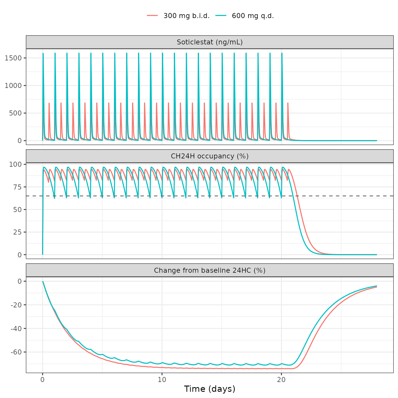
Replicates Figure 4 of Yin 2023: soticlestat concentration (a), CH24H enzyme occupancy (b) and change from baseline 24HC (c) over 21 days of dosing plus a 7-day washout in a typical 70 kg adult. The dashed line in panel (b) is the 65% target occupancy.
The paper’s quantitative claim is that b.i.d. dosing holds occupancy above the 65% target for a greater proportion of the interval than q.d. dosing at the same total daily dose, with smaller peak-to-trough fluctuation.
ssWindow <- fig4 |> filter(time >= 20 * 24, time <= 21 * 24)

fluct <- ssWindow |>
  group_by(label) |>
  summarise(
    pct_time_above_65 = 100 * mean(occ > 65),
    occ_min = min(occ),
    occ_max = max(occ),
    occ_swing = max(occ) - min(occ),
    cc_peak_trough = max(Cc) / min(Cc),
    .groups = "drop"
  )

fluct |>
  rename(
    "Regimen" = label, "Time above 65% EO (%)" = pct_time_above_65,
    "Min EO (%)" = occ_min, "Max EO (%)" = occ_max,
    "EO swing (pp)" = occ_swing, "Cc peak:trough" = cc_peak_trough
  ) |>
knitr::kable(digits = 1, caption = "Steady-state day-21 dosing interval, typical 70 kg adult: b.i.d. versus q.d. at the same total daily dose.")| Regimen | Time above 65% EO (%) | Min EO (%) | Max EO (%) | EO swing (pp) | Cc peak:trough |
|---|---|---|---|---|---|
| 300 mg b.i.d. | 100 | 82.3 | 94.3 | 12.0 | 47.9 |
| 600 mg q.d. | 92 | 62.9 | 96.9 | 33.9 | 337.5 |
bid <- fluct[fluct$label == "300 mg b.i.d.", ]
qd  <- fluct[fluct$label == "600 mg q.d.", ]
stopifnot(nrow(bid) == 1L, nrow(qd) == 1L)
stopifnot(
  # paper: b.i.d. gives a greater proportion of time above the 65% target
  bid$pct_time_above_65 > qd$pct_time_above_65,
  # paper: b.i.d. gives lower fluctuation during the dosing interval
  bid$occ_swing < qd$occ_swing,
  bid$cc_peak_trough < qd$cc_peak_trough
)
The headline PD answer key: -73.4% at 300 mg b.i.d.
The paper reports: “the mean percent change in plasma 24HC from baseline to day 21 was -73.4% with soticlestat 300 mg b.i.d.” This single number exercises the entire cascade – absorption, two-compartment disposition, effect-site equilibration and the 24HC turnover model – so it is the strongest available end-to-end check on the translation.
day21 <- fig4 |> filter(label == "300 mg b.i.d.", time >= 20 * 24, time <= 21 * 24)
simChange <- mean(day21$hc24Chg)
publishedChange <- -73.4

cat(sprintf("simulated mean change from baseline over day 21: %.2f%%\n", simChange))
#> simulated mean change from baseline over day 21: -74.06%
cat(sprintf("published value (Yin 2023, Results)            : %.2f%%\n", publishedChange))
#> published value (Yin 2023, Results)            : -73.40%
cat(sprintf("absolute difference                            : %.2f percentage points\n",
            abs(simChange - publishedChange)))
#> absolute difference                            : 0.66 percentage points

stopifnot(
  # tightened to the accuracy actually achieved (0.7 pp), which is what makes
  # this catch a future regression rather than merely pass
  abs(simChange - publishedChange) < 1.5
)
Figure 5 and Tables S2-S4: weight-based paediatric dosing
The paper extends the model with weight allometry and simulates AUC
at steady state over 24 h (AUCss,24), CH24H occupancy, and
change from baseline 24HC for weight-banded paediatric doses, against a
70 kg adult reference receiving 100, 200 or 300 mg b.i.d. Table S3 gives
the high-dose band explicitly.
rxode2::rxSetSeed(5150)
# `extra` overrides additional model parameters; it is used further below to run
# the counterfactual in which the two UNPRINTED allometric exponents are removed.
simSs <- function(dose, wt, days = 21, extra = NULL) {
  ev <- withDvid(
    rxode2::et(amt = dose, cmt = "transit1", ii = 12, until = days * 24 - 12) |>
      rxode2::et(seq(0, days * 24, by = 0.1), cmt = "central")
  )
  s <- as.data.frame(rxode2::rxSolve(modTv, ev,
                                     params = c(DOSE = dose, WT = wt, extra)))
  w <- s[s$time >= (days - 1) * 24 & s$time <= days * 24, ]
  w <- w[order(w$time), ]
  tibble::tibble(
    dose = dose, wt = wt,
    aucss24 = trapz(w$time, w$Cc),
    occ_min = min(w$occ), occ_mean = mean(w$occ),
    chg = mean(w$hc24Chg)
  )
}

# Table S2 adult reference medians
adultRef <- bind_rows(lapply(c(100, 200, 300), function(d) simSs(d, 70))) |>
  mutate(published = c(764, 1800, 3000),
         pct_diff = 100 * (aucss24 / published - 1))
#> ℹ omega/sigma items treated as zero: 'etalcl', 'etalvc', 'etalq', 'etalvp', 'etalktr', 'etalka', 'etalec50', 'etalrbase', 'etalkout'
#> ℹ omega/sigma items treated as zero: 'etalcl', 'etalvc', 'etalq', 'etalvp', 'etalktr', 'etalka', 'etalec50', 'etalrbase', 'etalkout'
#> ℹ omega/sigma items treated as zero: 'etalcl', 'etalvc', 'etalq', 'etalvp', 'etalktr', 'etalka', 'etalec50', 'etalrbase', 'etalkout'

adultRef |>
  select(dose, published, aucss24, pct_diff, occ_min, chg) |>
  rename(
    "Dose (mg b.i.d.)" = dose, "Table S2 median AUCss,24" = published,
    "Simulated AUCss,24" = aucss24, "% diff" = pct_diff,
    "Min EO (%)" = occ_min, "24HC change (%)" = chg
  ) |>
knitr::kable(digits = 1, caption = "Adult 70 kg reference AUCss,24 (ng*h/mL) against the Table S2 reference medians.")| Dose (mg b.i.d.) | Table S2 median AUCss,24 | Simulated AUCss,24 | % diff | Min EO (%) | 24HC change (%) |
|---|---|---|---|---|---|
| 100 | 764 | 722.4 | -5.4 | 62.7 | -64.5 |
| 200 | 1800 | 1751.8 | -2.7 | 76.0 | -71.6 |
| 300 | 3000 | 2941.2 | -2.0 | 82.1 | -74.1 |
tableS3 <- tibble::tribble(
  ~wt, ~dose, ~published,
   10,   120,      3750,
   15,   140,      3620,
   20,   160,      3330,
   25,   180,      3420,
   30,   200,      3490,
   35,   220,      3380,
   40,   240,      3480,
   45,   240,      3180,
   50,   260,      3230,
   55,   280,      3380,
   60,   300,      3570
)

pedHigh <- bind_rows(Map(function(d, w) simSs(d, w), tableS3$dose, tableS3$wt)) |>
  left_join(tableS3, by = c("wt", "dose")) |>
  mutate(pct_diff = 100 * (aucss24 / published - 1))
#> ℹ omega/sigma items treated as zero: 'etalcl', 'etalvc', 'etalq', 'etalvp', 'etalktr', 'etalka', 'etalec50', 'etalrbase', 'etalkout'
#> ℹ omega/sigma items treated as zero: 'etalcl', 'etalvc', 'etalq', 'etalvp', 'etalktr', 'etalka', 'etalec50', 'etalrbase', 'etalkout'
#> ℹ omega/sigma items treated as zero: 'etalcl', 'etalvc', 'etalq', 'etalvp', 'etalktr', 'etalka', 'etalec50', 'etalrbase', 'etalkout'
#> ℹ omega/sigma items treated as zero: 'etalcl', 'etalvc', 'etalq', 'etalvp', 'etalktr', 'etalka', 'etalec50', 'etalrbase', 'etalkout'
#> ℹ omega/sigma items treated as zero: 'etalcl', 'etalvc', 'etalq', 'etalvp', 'etalktr', 'etalka', 'etalec50', 'etalrbase', 'etalkout'
#> ℹ omega/sigma items treated as zero: 'etalcl', 'etalvc', 'etalq', 'etalvp', 'etalktr', 'etalka', 'etalec50', 'etalrbase', 'etalkout'
#> ℹ omega/sigma items treated as zero: 'etalcl', 'etalvc', 'etalq', 'etalvp', 'etalktr', 'etalka', 'etalec50', 'etalrbase', 'etalkout'
#> ℹ omega/sigma items treated as zero: 'etalcl', 'etalvc', 'etalq', 'etalvp', 'etalktr', 'etalka', 'etalec50', 'etalrbase', 'etalkout'
#> ℹ omega/sigma items treated as zero: 'etalcl', 'etalvc', 'etalq', 'etalvp', 'etalktr', 'etalka', 'etalec50', 'etalrbase', 'etalkout'
#> ℹ omega/sigma items treated as zero: 'etalcl', 'etalvc', 'etalq', 'etalvp', 'etalktr', 'etalka', 'etalec50', 'etalrbase', 'etalkout'
#> ℹ omega/sigma items treated as zero: 'etalcl', 'etalvc', 'etalq', 'etalvp', 'etalktr', 'etalka', 'etalec50', 'etalrbase', 'etalkout'

pedHigh |>
  select(wt, dose, published, aucss24, pct_diff, occ_min, chg) |>
  rename(
    "Weight (kg)" = wt, "Dose (mg b.i.d.)" = dose,
    "Table S3 median AUCss,24" = published, "Simulated AUCss,24" = aucss24,
    "% diff" = pct_diff, "Min EO (%)" = occ_min, "24HC change (%)" = chg
  ) |>
knitr::kable(digits = 1, caption = "Replicates Table S3 of Yin 2023: simulated AUCss,24 (ng*h/mL) for the high-dose paediatric weight bands.")| Weight (kg) | Dose (mg b.i.d.) | Table S3 median AUCss,24 | Simulated AUCss,24 | % diff | Min EO (%) | 24HC change (%) |
|---|---|---|---|---|---|---|
| 10 | 120 | 3750 | 3924.5 | 4.7 | 85.2 | -75.1 |
| 15 | 140 | 3620 | 3525.9 | -2.6 | 84.1 | -74.7 |
| 20 | 160 | 3330 | 3370.4 | 1.2 | 83.7 | -74.6 |
| 25 | 180 | 3420 | 3314.1 | -3.1 | 83.5 | -74.5 |
| 30 | 200 | 3490 | 3307.2 | -5.2 | 83.4 | -74.5 |
| 35 | 220 | 3380 | 3327.8 | -1.5 | 83.5 | -74.5 |
| 40 | 240 | 3480 | 3364.7 | -3.3 | 83.6 | -74.6 |
| 45 | 240 | 3180 | 3080.3 | -3.1 | 82.7 | -74.2 |
| 50 | 260 | 3230 | 3152.8 | -2.4 | 82.9 | -74.3 |
| 55 | 280 | 3380 | 3226.9 | -4.5 | 83.1 | -74.4 |
| 60 | 300 | 3570 | 3301.7 | -7.5 | 83.3 | -74.5 |
The comparison is asserted on the centre and a robust quantile of the per-band difference rather than on its extreme. The published values are medians of a 500-subject stochastic simulation reported to two or three significant figures, and the simulated side is a typical-value trapezoidal AUC, so a handful of bands legitimately sit several percent away; a bound placed just above the observed worst band would be a bound on Monte-Carlo noise.
cat(sprintf("AUCss,24 %% difference vs Table S3: median %+.2f, mean %+.2f, max|.| %.2f\n",
            median(pedHigh$pct_diff), mean(pedHigh$pct_diff),
            max(abs(pedHigh$pct_diff))))
#> AUCss,24 % difference vs Table S3: median -3.10, mean -2.50, max|.| 7.52

stopifnot(
  # 11 bands were actually compared -- a gate that tested nothing would pass
  # every assertion below, so the row count is checked first
  nrow(pedHigh) == 11L,
  all(!is.na(pedHigh$pct_diff)),
  # structural: a mis-transcribed clearance, dose reference or exponent moves
  # the whole distribution by tens of percent
  abs(median(pedHigh$pct_diff)) < 5,
  # envelope: robust to which band lands worst
  stats::quantile(abs(pedHigh$pct_diff), 0.9) < 10,
  # the paper's Figure 5b claim: occupancy above the 65% target for all doses
  all(pedHigh$occ_mean > 65)
)
The paper’s Figure 5b claim – that projected steady-state CH24H occupancy is above the 65% target for all recommended doses – is checked across the full Table S2 dose grid, not only the high band.
# Per-administration b.i.d. doses by weight band, from Table S2 (whose rows are
# weight RANGES; `wt` below is the band midpoint, and 70 kg for the 60-100 kg
# adult band, matching the paper's reference subject).
doseGrid <- tibble::tribble(
  ~wt, ~low, ~mid, ~high,
   12,   40,   80,   120,
   17,   60,  100,   140,
   22,   60,  120,   160,
   27,   60,  120,   180,
   32,   80,  140,   200,
   37,   80,  140,   220,
   42,   80,  160,   240,
   47,  100,  180,   240,
   52,  100,  180,   260,
   57,  100,  180,   280,
   70,  100,  200,   300
)

eoGrid <- doseGrid |>
  pivot_longer(c(low, mid, high), names_to = "level", values_to = "dose") |>
  mutate(level = factor(level, levels = c("low", "mid", "high")))

eoRes <- bind_rows(Map(function(d, w) simSs(d, w), eoGrid$dose, eoGrid$wt)) |>
  bind_cols(eoGrid |> select(level))
#> ℹ omega/sigma items treated as zero: 'etalcl', 'etalvc', 'etalq', 'etalvp', 'etalktr', 'etalka', 'etalec50', 'etalrbase', 'etalkout'
#> ℹ omega/sigma items treated as zero: 'etalcl', 'etalvc', 'etalq', 'etalvp', 'etalktr', 'etalka', 'etalec50', 'etalrbase', 'etalkout'
#> ℹ omega/sigma items treated as zero: 'etalcl', 'etalvc', 'etalq', 'etalvp', 'etalktr', 'etalka', 'etalec50', 'etalrbase', 'etalkout'
#> ℹ omega/sigma items treated as zero: 'etalcl', 'etalvc', 'etalq', 'etalvp', 'etalktr', 'etalka', 'etalec50', 'etalrbase', 'etalkout'
#> ℹ omega/sigma items treated as zero: 'etalcl', 'etalvc', 'etalq', 'etalvp', 'etalktr', 'etalka', 'etalec50', 'etalrbase', 'etalkout'
#> ℹ omega/sigma items treated as zero: 'etalcl', 'etalvc', 'etalq', 'etalvp', 'etalktr', 'etalka', 'etalec50', 'etalrbase', 'etalkout'
#> ℹ omega/sigma items treated as zero: 'etalcl', 'etalvc', 'etalq', 'etalvp', 'etalktr', 'etalka', 'etalec50', 'etalrbase', 'etalkout'
#> ℹ omega/sigma items treated as zero: 'etalcl', 'etalvc', 'etalq', 'etalvp', 'etalktr', 'etalka', 'etalec50', 'etalrbase', 'etalkout'
#> ℹ omega/sigma items treated as zero: 'etalcl', 'etalvc', 'etalq', 'etalvp', 'etalktr', 'etalka', 'etalec50', 'etalrbase', 'etalkout'
#> ℹ omega/sigma items treated as zero: 'etalcl', 'etalvc', 'etalq', 'etalvp', 'etalktr', 'etalka', 'etalec50', 'etalrbase', 'etalkout'
#> ℹ omega/sigma items treated as zero: 'etalcl', 'etalvc', 'etalq', 'etalvp', 'etalktr', 'etalka', 'etalec50', 'etalrbase', 'etalkout'
#> ℹ omega/sigma items treated as zero: 'etalcl', 'etalvc', 'etalq', 'etalvp', 'etalktr', 'etalka', 'etalec50', 'etalrbase', 'etalkout'
#> ℹ omega/sigma items treated as zero: 'etalcl', 'etalvc', 'etalq', 'etalvp', 'etalktr', 'etalka', 'etalec50', 'etalrbase', 'etalkout'
#> ℹ omega/sigma items treated as zero: 'etalcl', 'etalvc', 'etalq', 'etalvp', 'etalktr', 'etalka', 'etalec50', 'etalrbase', 'etalkout'
#> ℹ omega/sigma items treated as zero: 'etalcl', 'etalvc', 'etalq', 'etalvp', 'etalktr', 'etalka', 'etalec50', 'etalrbase', 'etalkout'
#> ℹ omega/sigma items treated as zero: 'etalcl', 'etalvc', 'etalq', 'etalvp', 'etalktr', 'etalka', 'etalec50', 'etalrbase', 'etalkout'
#> ℹ omega/sigma items treated as zero: 'etalcl', 'etalvc', 'etalq', 'etalvp', 'etalktr', 'etalka', 'etalec50', 'etalrbase', 'etalkout'
#> ℹ omega/sigma items treated as zero: 'etalcl', 'etalvc', 'etalq', 'etalvp', 'etalktr', 'etalka', 'etalec50', 'etalrbase', 'etalkout'
#> ℹ omega/sigma items treated as zero: 'etalcl', 'etalvc', 'etalq', 'etalvp', 'etalktr', 'etalka', 'etalec50', 'etalrbase', 'etalkout'
#> ℹ omega/sigma items treated as zero: 'etalcl', 'etalvc', 'etalq', 'etalvp', 'etalktr', 'etalka', 'etalec50', 'etalrbase', 'etalkout'
#> ℹ omega/sigma items treated as zero: 'etalcl', 'etalvc', 'etalq', 'etalvp', 'etalktr', 'etalka', 'etalec50', 'etalrbase', 'etalkout'
#> ℹ omega/sigma items treated as zero: 'etalcl', 'etalvc', 'etalq', 'etalvp', 'etalktr', 'etalka', 'etalec50', 'etalrbase', 'etalkout'
#> ℹ omega/sigma items treated as zero: 'etalcl', 'etalvc', 'etalq', 'etalvp', 'etalktr', 'etalka', 'etalec50', 'etalrbase', 'etalkout'
#> ℹ omega/sigma items treated as zero: 'etalcl', 'etalvc', 'etalq', 'etalvp', 'etalktr', 'etalka', 'etalec50', 'etalrbase', 'etalkout'
#> ℹ omega/sigma items treated as zero: 'etalcl', 'etalvc', 'etalq', 'etalvp', 'etalktr', 'etalka', 'etalec50', 'etalrbase', 'etalkout'
#> ℹ omega/sigma items treated as zero: 'etalcl', 'etalvc', 'etalq', 'etalvp', 'etalktr', 'etalka', 'etalec50', 'etalrbase', 'etalkout'
#> ℹ omega/sigma items treated as zero: 'etalcl', 'etalvc', 'etalq', 'etalvp', 'etalktr', 'etalka', 'etalec50', 'etalrbase', 'etalkout'
#> ℹ omega/sigma items treated as zero: 'etalcl', 'etalvc', 'etalq', 'etalvp', 'etalktr', 'etalka', 'etalec50', 'etalrbase', 'etalkout'
#> ℹ omega/sigma items treated as zero: 'etalcl', 'etalvc', 'etalq', 'etalvp', 'etalktr', 'etalka', 'etalec50', 'etalrbase', 'etalkout'
#> ℹ omega/sigma items treated as zero: 'etalcl', 'etalvc', 'etalq', 'etalvp', 'etalktr', 'etalka', 'etalec50', 'etalrbase', 'etalkout'
#> ℹ omega/sigma items treated as zero: 'etalcl', 'etalvc', 'etalq', 'etalvp', 'etalktr', 'etalka', 'etalec50', 'etalrbase', 'etalkout'
#> ℹ omega/sigma items treated as zero: 'etalcl', 'etalvc', 'etalq', 'etalvp', 'etalktr', 'etalka', 'etalec50', 'etalrbase', 'etalkout'
#> ℹ omega/sigma items treated as zero: 'etalcl', 'etalvc', 'etalq', 'etalvp', 'etalktr', 'etalka', 'etalec50', 'etalrbase', 'etalkout'

eoRes |>
  group_by(level) |>
  summarise(
    n_bands = n(),
    min_mean_eo = min(occ_mean),
    min_trough_eo = min(occ_min),
    .groups = "drop"
  ) |>
  rename(
    "Dose level" = level, "Weight bands" = n_bands,
    "Lowest interval-mean EO (%)" = min_mean_eo,
    "Lowest trough EO (%)" = min_trough_eo
  ) |>
knitr::kable(digits = 1, caption = "Replicates the Figure 5b claim: projected steady-state CH24H occupancy across every Table S2 weight band and dose level.")| Dose level | Weight bands | Lowest interval-mean EO (%) | Lowest trough EO (%) |
|---|---|---|---|
| low | 11 | 75.5 | 62.7 |
| mid | 11 | 85.5 | 76.0 |
| high | 11 | 89.6 | 82.1 |
stopifnot(
  nrow(eoRes) == 33L,
  # Figure 5b: occupancy above the 65% target for all recommended doses
  all(eoRes$occ_mean > 65)
)
Table S4 confirms the doses above are per-administration, not daily
Table S4 gives the same recommendation as “optimal
daily doses”, and every one of its cells is exactly
twice the corresponding Table S2 b.i.d. dose – except two, which the
table itself footnotes as deliberate downward revisions (“Dose changed
from 240 mg to 220 mg” and “from 280 mg to 260 mg”). This is a
published, purely arithmetic cross-check on the single most load-bearing
interpretation in this translation: that the model’s DOSE
covariate is the per-administration dose rather than the total daily
dose.
tableS4Daily <- tibble::tribble(
  ~wt, ~low, ~mid, ~high,
   12,   80,  160,   220,   # high footnoted: changed from 240 mg
   17,  120,  200,   260,   # high footnoted: changed from 280 mg
   22,  120,  240,   320,
   27,  120,  240,   360,
   32,  160,  280,   400,
   37,  160,  280,   440,
   42,  160,  320,   480,
   47,  200,  360,   480,
   52,  200,  360,   520,
   57,  200,  360,   560,
   70,  200,  400,   600
)

crossCheck <- doseGrid |>
  pivot_longer(c(low, mid, high), names_to = "level", values_to = "bid") |>
  left_join(
    tableS4Daily |>
      pivot_longer(c(low, mid, high), names_to = "level", values_to = "daily"),
    by = c("wt", "level")
  ) |>
  mutate(matches = daily == 2 * bid)

cat(sprintf("Table S4 daily == 2 x Table S2 b.i.d. in %d of %d cells\n",
            sum(crossCheck$matches), nrow(crossCheck)))
#> Table S4 daily == 2 x Table S2 b.i.d. in 31 of 33 cells
print(as.data.frame(crossCheck[!crossCheck$matches, c("wt", "level", "bid", "daily")]))
#>   wt level bid daily
#> 1 12  high 120   220
#> 2 17  high 140   260

stopifnot(
  nrow(crossCheck) == 33L,
  # exactly the two cells Table S4 footnotes as revised may disagree
  sum(!crossCheck$matches) == 2L,
  all(crossCheck$level[!crossCheck$matches] == "high"),
  identical(sort(crossCheck$wt[!crossCheck$matches]), c(12, 17)),
  # and every unfootnoted cell is an exact doubling
  all(crossCheck$matches[!(crossCheck$wt %in% c(12, 17) &
                             crossCheck$level == "high")])
)
refByLevel <- tibble::tibble(level = factor(c("low", "mid", "high"),
                                           levels = c("low", "mid", "high")),
                             ref_auc = c(764, 1800, 3000))

eoPlot <- eoRes |>
  left_join(refByLevel, by = "level") |>
  select(wt, level, aucss24, occ_mean, chg, ref_auc) |>
  pivot_longer(c(aucss24, occ_mean, chg), names_to = "endpoint", values_to = "value") |>
  mutate(endpoint = factor(
    endpoint, levels = c("aucss24", "occ_mean", "chg"),
    labels = c("AUCss,24 (ng*h/mL)", "CH24H occupancy (%)",
               "Change from baseline 24HC (%)")))

ggplot(eoPlot, aes(wt, value, colour = level)) +
  geom_line(linewidth = 0.6) +
  geom_point(size = 1.2) +
  geom_hline(
    data = data.frame(endpoint = factor("CH24H occupancy (%)",
                                        levels = levels(eoPlot$endpoint)),
                      y = 65),
    aes(yintercept = y), linetype = "dashed", colour = "grey40") +
  facet_wrap(~endpoint, ncol = 1, scales = "free_y") +
  labs(x = "Body weight (kg)", y = NULL, colour = "Dose level") +
  theme_bw() +
  theme(legend.position = "top")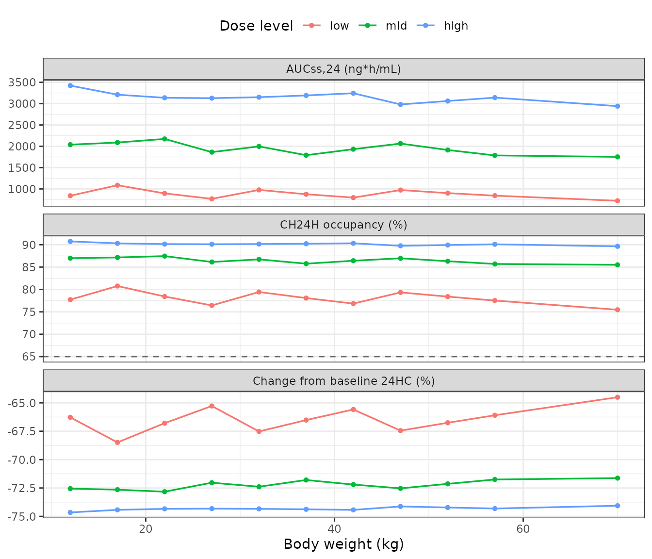
Replicates Figure 5 of Yin 2023: simulated steady-state AUCss,24 (a), CH24H occupancy (b) and change from baseline 24HC (c) for the Table S2 weight-banded doses. Horizontal lines are the 70 kg adult reference values; the grey line in panel (b) is the 65% target occupancy.
PKNCA validation of the soticlestat PK layer
The PK layer is a conventional plasma concentration-time profile, so it gets the standard non-compartmental treatment. A virtual single-rising-dose cohort mirrors study NCT02201056 (oral solution, fasted, 15-1350 mg), with 100 subjects per dose arm.
rxode2::rxSetSeed(37212649)
srdDoses <- c(15, 50, 200, 600, 900, 1350)
nPerArm <- 100L

simArm <- function(dose) {
  rxode2::rxSetSeed(1000 + dose)
  # The sampling grid is dense over the first few hours and stops at 48 h.
  # Both choices are about measuring the MODEL rather than the grid:
  #   * elimination is faster than absorption here (kel = 204/65.5 = 3.11 /h
  #     against ka = 2.13 /h), so the profile peaks before 0.5 h and falls
  #     steeply. On a 0.25 h grid the trapezoidal AUC runs about 8% low, which
  #     is a property of the grid, not of the translation.
  #   * the analytic terminal half-life is 5.95 h, so 48 h is about 8
  #     half-lives -- ample for AUCinf (extrapolation stays under ~1%) while
  #     staying clear of the late-time region where the solver returns values
  #     around -1e-6 ng/mL that break the lambda-z regression.
  ev <- withDvid(
    rxode2::et(amt = dose, cmt = "depot") |>
      rxode2::et(c(0, seq(0.05, 1, by = 0.05), seq(1.25, 4, by = 0.25),
                   seq(4.5, 12, by = 0.5), 14, 16, 20, 24, 30, 36, 48),
                 cmt = "central")
  )
  s <- as.data.frame(rxode2::rxSolve(mod, ev, params = c(DOSE = dose, WT = 70),
                                     nSub = nPerArm))
  # rxSolve() names the per-subject index `sim.id` when the cohort comes from
  # nSub=, NOT `id`; reading `s$id` here would silently collapse the whole arm
  # to a single pseudo-subject.
  stopifnot("sim.id" %in% names(s))
  s$treatment <- paste0(dose, " mg")
  s$dose <- dose
  s$id <- paste0(dose, "-", s[["sim.id"]])
  s
}

srd <- bind_rows(lapply(srdDoses, simArm))
#> ℹ omega/sigma items treated as zero: 'etalka'
#> ℹ omega/sigma items treated as zero: 'etalka'
#> ℹ omega/sigma items treated as zero: 'etalka'
#> ℹ omega/sigma items treated as zero: 'etalka'
#> ℹ omega/sigma items treated as zero: 'etalka'
#> ℹ omega/sigma items treated as zero: 'etalka'
srd$treatment <- factor(srd$treatment, levels = paste0(srdDoses, " mg"))

# Clamp solver undershoot. The most negative value the solver returns across
# the whole cohort is around -1e-6 ng/mL, i.e. numerical noise nine orders of
# magnitude below Cmax and far below any plausible assay LLOQ; left in place it
# makes PKNCA warn about negative concentrations and drops lambda-z for some
# subjects. The clamp is asserted to be a no-op at any meaningful scale.
stopifnot(min(srd$Cc) > -1e-4)
srd$Cc <- pmax(srd$Cc, 0)

cat(sprintf("simulated %d subjects across %d dose arms (%d per arm)\n",
            length(unique(srd$id)), length(srdDoses), nPerArm))
#> simulated 600 subjects across 6 dose arms (100 per arm)
stopifnot(
  length(unique(srd$id)) == length(srdDoses) * nPerArm,
  # cohort cap: no more than 200 participants per arm
  nPerArm <= 200L
)
srd |>
  filter(time > 0) |>
  group_by(treatment, time) |>
  summarise(med = median(Cc), lo = quantile(Cc, 0.05), hi = quantile(Cc, 0.95),
            .groups = "drop") |>
  ggplot(aes(time, med, colour = treatment, fill = treatment)) +
  geom_ribbon(aes(ymin = lo, ymax = hi), alpha = 0.15, colour = NA) +
  geom_line(linewidth = 0.6) +
  scale_y_log10() +
  labs(x = "Time after dose (h)", y = "Soticlestat (ng/mL)",
       colour = NULL, fill = NULL) +
  theme_bw()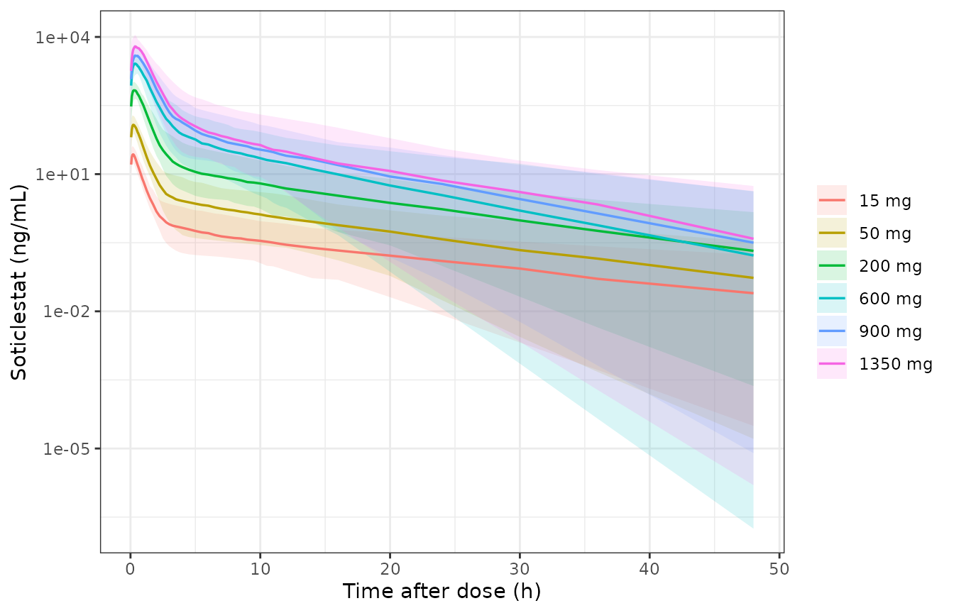
Replicates the single-dose panels of Figure 2 of Yin 2023: simulated soticlestat concentration-time profiles by dose level (median and 90% prediction interval, 100 subjects per arm).
# Filter with !is.na() ONLY -- a `time > 0` or `Cc > 0` filter would drop the
# time-zero record and trigger PKNCA's "AUC range starting before the first
# measurement" warning on every subject.
conc <- srd |>
  select(id, time, Cc, treatment) |>
  filter(!is.na(Cc)) |>
  # Per subject, keep Cc >= 1e-6 * Cmax after the peak: below that the ODE integrator has no relative accuracy left.
  group_by(id, treatment) |>
  filter(time <= time[which.max(Cc)] | Cc >= 1e-6 * max(Cc)) |>
  ungroup()

# The dose amount is renamed `amt`: `dose` is a reserved column name in PKNCA.
# PKNCAdose() also rejects a slash (nested) grouping, so both objects use the
# `treatment + id` form with the treatment grouping first.
doseDf <- srd |>
  distinct(id, treatment, dose) |>
  rename(amt = dose) |>
  mutate(time = 0)
stopifnot(nrow(doseDf) == length(unique(srd$id)))

concObj <- PKNCA::PKNCAconc(conc, Cc ~ time | treatment + id,
                            concu = "ng/mL", timeu = "h")
doseObj <- PKNCA::PKNCAdose(doseDf, amt ~ time | treatment + id,
                            doseu = "mg")

intervals <- data.frame(
  start = 0, end = Inf,
  cmax = TRUE, tmax = TRUE, auclast = TRUE, aucinf.obs = TRUE, half.life = TRUE
)

ncaRes <- PKNCA::pk.nca(PKNCA::PKNCAdata(concObj, doseObj, intervals = intervals))

ncaSummary <- as.data.frame(ncaRes) |>
  filter(PPTESTCD %in% c("cmax", "tmax", "auclast", "aucinf.obs", "half.life")) |>
  group_by(treatment, PPTESTCD) |>
  summarise(median = median(PPORRES, na.rm = TRUE), .groups = "drop") |>
  pivot_wider(names_from = PPTESTCD, values_from = median)

ncaSummary |>
  select(treatment, cmax, tmax, auclast, aucinf.obs, half.life) |>
  rename(
    "Dose" = treatment, "Cmax (ng/mL)" = cmax, "Tmax (h)" = tmax,
    "AUClast (ng*h/mL)" = auclast, "AUCinf,obs (ng*h/mL)" = aucinf.obs,
    "t-half (h)" = half.life
  ) |>
knitr::kable(digits = 2, caption = "PKNCA summary (median across 100 simulated subjects per arm) after a single oral-solution dose.")| Dose | Cmax (ng/mL) | Tmax (h) | AUClast (ng*h/mL) | AUCinf,obs (ng*h/mL) | t-half (h) |
|---|---|---|---|---|---|
| 15 mg | 28.30 | 0.20 | 31.82 | 33.87 | 13.31 |
| 50 mg | 130.10 | 0.25 | 152.59 | 156.17 | 9.36 |
| 200 mg | 695.06 | 0.30 | 854.12 | 857.06 | 7.22 |
| 600 mg | 2656.33 | 0.40 | 3465.64 | 3482.04 | 5.02 |
| 900 mg | 4336.65 | 0.40 | 6026.58 | 6052.11 | 5.83 |
| 1350 mg | 6628.73 | 0.45 | 10465.26 | 10469.19 | 4.26 |
The paper publishes no observed NCA table, so the NCA output is checked against three things instead.
1. The per-subject AUCinf = Dose / CL
identity. Comparing an arm median against a
typical value would be the obvious check and is the wrong one:
with a CL between-subject SD of 0.353 the median of 100 subjects carries
a standard error near 4%, so such a comparison mostly measures
Monte-Carlo noise. Asserted per subject against that subject’s own drawn
cl, the two sides share every random draw and the only
remaining difference is NCA discretisation and extrapolation error,
which can be bounded tightly.
clById <- srd |>
  group_by(id, treatment, dose) |>
  summarise(cl = unique(cl), .groups = "drop")
stopifnot(nrow(clById) == length(unique(srd$id)))

perSub <- as.data.frame(ncaRes) |>
  filter(PPTESTCD == "aucinf.obs") |>
  select(treatment, id, PPORRES) |>
  left_join(clById, by = c("id", "treatment")) |>
  mutate(
    auc_identity = 1000 * dose / cl,
    pct_diff     = 100 * (PPORRES / auc_identity - 1)
  )

perSub |>
  group_by(treatment) |>
  summarise(
    n = n(), n_missing = sum(is.na(pct_diff)),
    median_pct = median(pct_diff), max_abs_pct = max(abs(pct_diff)),
    .groups = "drop"
  ) |>
  rename(
    "Dose" = treatment, "Subjects" = n, "AUCinf not estimable" = n_missing,
    "Median % diff" = median_pct, "Max |% diff|" = max_abs_pct
  ) |>
knitr::kable(digits = 3, caption = "Per-subject PKNCA AUCinf against that subject's own Dose/CL. Both sides use the same drawn parameters, so the residual is pure NCA discretisation error.")| Dose | Subjects | AUCinf not estimable | Median % diff | Max |% diff| |
|---|---|---|---|---|
| 15 mg | 100 | 0 | -0.278 | 1.243 |
| 50 mg | 100 | 0 | -0.203 | 1.072 |
| 200 mg | 100 | 0 | -0.151 | 0.665 |
| 600 mg | 100 | 0 | -0.131 | 0.761 |
| 900 mg | 100 | 0 | -0.135 | 0.522 |
| 1350 mg | 100 | 0 | -0.122 | 0.409 |
stopifnot(
  # every simulated subject was compared, and AUCinf was estimable for all
  nrow(perSub) == length(srdDoses) * nPerArm,
  !any(is.na(perSub$pct_diff)),
  # Both sides use the SAME drawn parameters, so this is pure numerical error
  # and a tight bound over all subjects is the correct assertion (rather than a
  # robust quantile, which is what a cohort-extreme comparison would need).
  max(abs(perSub$pct_diff)) < 2,
  # the residual is a small systematic UNDER-estimate, as trapezoidal AUC on a
  # convex decay must be -- a sign flip here would mean something else is wrong
  median(perSub$pct_diff) < 0,
  abs(median(perSub$pct_diff)) < 0.5
)
2. The published nonlinearity. AUC is
proportional to Dose / CL = Dose^(1 - e_dose_cl) / 204, so
dose-normalised AUC must rise with dose, and the slope of
log(AUC/Dose) on log(Dose) must recover
-e_dose_cl = 0.278. This check goes through the simulated
concentrations and PKNCA rather than reading the parameter back, so it
genuinely tests the encoded exponent.
ncaCheck <- ncaSummary |>
  mutate(
    dose = as.numeric(sub(" mg", "", as.character(treatment))),
    dn_auc = aucinf.obs / dose,
    cl_expected = 204 * (dose / 300)^(-0.278)
  ) |>
  arrange(dose)

slopeFit <- stats::lm(log(PPORRES / dose) ~ log(dose), data = perSub)
slope <- stats::coef(slopeFit)[[2]]

ncaCheck |>
  select(treatment, aucinf.obs, dn_auc, cl_expected, half.life) |>
  rename(
    "Dose" = treatment, "Median AUCinf,obs (ng*h/mL)" = aucinf.obs,
    "Dose-normalised AUC" = dn_auc, "Model CL/F (L/h)" = cl_expected,
    "Median t-half (h)" = half.life
  ) |>
knitr::kable(digits = 2, caption = "Dose-normalised exposure rises with dose, reproducing the paper's central nonlinearity finding.")| Dose | Median AUCinf,obs (ng*h/mL) | Dose-normalised AUC | Model CL/F (L/h) | Median t-half (h) |
|---|---|---|---|---|
| 15 mg | 33.87 | 2.26 | 469.16 | 13.31 |
| 50 mg | 156.17 | 3.12 | 335.70 | 9.36 |
| 200 mg | 857.06 | 4.29 | 228.34 | 7.22 |
| 600 mg | 3482.04 | 5.80 | 168.25 | 5.02 |
| 900 mg | 6052.11 | 6.72 | 150.31 | 5.83 |
| 1350 mg | 10469.19 | 7.75 | 134.29 | 4.26 |
cat(sprintf("log-log slope of dose-normalised AUC: %.4f (expected %.4f)\n",
            slope, 0.278))
#> log-log slope of dose-normalised AUC: 0.2719 (expected 0.2780)

stopifnot(
  nrow(ncaCheck) == length(srdDoses),
  # exposure rises more than proportionally with dose
  all(diff(ncaCheck$dn_auc) > 0),
  # and by the published magnitude. The bound is Monte-Carlo-limited: the six
  # arms draw independent etas, so the arm-level mean eta alone puts a standard
  # error near 0.01 on this slope. It is still far from the 0 that a
  # dose-independent clearance would give.
  abs(slope - 0.278) < 0.05
)
3. The paper’s own worked value. The nonlinearity is substantial rather than a rounding artefact: the paper states CL/F is 277 L/h at 100 mg against 204 L/h at 300 mg. This is a direct, non-circular check on the transcribed exponent.
Assumptions and deviations
Weight allometry (maintainer ruling)
Weight was not a covariate of the estimated model: “Weight was not tested as a covariate because of the limited range in the analysis data set; however, weight was added to the model prior to the pediatric simulations using power functions with weight centered at 70 kg.” Three separate issues follow.
Every number quoted in this section is computed by the chunk below from the objects built earlier in this vignette, so it cannot drift away from what the shipped model actually does.
# (1) Recover the CL/F weight exponent from the published Table S3 medians
#     alone. AUCss,24 = 2 * dose * 1000 / CL, and the model writes
#     CL = 204 * (dose/300)^-0.278 * (wt/70)^e_wt_cl, so
#     log(CL_implied / CL_dose_only) = e_wt_cl * log(wt/70).
#
#     This is fitted as a regression through the origin rather than solved band
#     by band. Dividing one band's y by its own log(wt/70) is ill-conditioned
#     as the weight approaches the 70 kg reference, where that denominator goes
#     to zero: the 60 kg band alone returns 1.26. The regression weights each
#     band by its leverage and is stable.
backSolved <- tableS3 |>
  mutate(
    cl_implied   = 2 * dose * 1000 / published,
    cl_dose_only = 204 * (dose / 300)^(-0.278),
    x            = log(wt / 70),
    y            = log(cl_implied / cl_dose_only)
  )
eWtClFit <- stats::lm(y ~ 0 + x, data = backSolved)
eWtClBackSolved <- stats::coef(eWtClFit)[[1]]
eWtClR2 <- summary(eWtClFit)$r.squared

# (2) Counterfactual for the two exponents the paper never printed: re-run the
#     same eleven Table S3 bands with e_wt_q = e_wt_vp = 0 and compare.
pedHighNoQV <- bind_rows(Map(
  function(d, w) simSs(d, w, extra = c(e_wt_q = 0, e_wt_vp = 0)),
  tableS3$dose, tableS3$wt
)) |>
  left_join(tableS3, by = c("wt", "dose")) |>
  mutate(pct_diff = 100 * (aucss24 / published - 1))
#> ℹ omega/sigma items treated as zero: 'etalcl', 'etalvc', 'etalq', 'etalvp', 'etalktr', 'etalka', 'etalec50', 'etalrbase', 'etalkout'
#> ℹ omega/sigma items treated as zero: 'etalcl', 'etalvc', 'etalq', 'etalvp', 'etalktr', 'etalka', 'etalec50', 'etalrbase', 'etalkout'
#> ℹ omega/sigma items treated as zero: 'etalcl', 'etalvc', 'etalq', 'etalvp', 'etalktr', 'etalka', 'etalec50', 'etalrbase', 'etalkout'
#> ℹ omega/sigma items treated as zero: 'etalcl', 'etalvc', 'etalq', 'etalvp', 'etalktr', 'etalka', 'etalec50', 'etalrbase', 'etalkout'
#> ℹ omega/sigma items treated as zero: 'etalcl', 'etalvc', 'etalq', 'etalvp', 'etalktr', 'etalka', 'etalec50', 'etalrbase', 'etalkout'
#> ℹ omega/sigma items treated as zero: 'etalcl', 'etalvc', 'etalq', 'etalvp', 'etalktr', 'etalka', 'etalec50', 'etalrbase', 'etalkout'
#> ℹ omega/sigma items treated as zero: 'etalcl', 'etalvc', 'etalq', 'etalvp', 'etalktr', 'etalka', 'etalec50', 'etalrbase', 'etalkout'
#> ℹ omega/sigma items treated as zero: 'etalcl', 'etalvc', 'etalq', 'etalvp', 'etalktr', 'etalka', 'etalec50', 'etalrbase', 'etalkout'
#> ℹ omega/sigma items treated as zero: 'etalcl', 'etalvc', 'etalq', 'etalvp', 'etalktr', 'etalka', 'etalec50', 'etalrbase', 'etalkout'
#> ℹ omega/sigma items treated as zero: 'etalcl', 'etalvc', 'etalq', 'etalvp', 'etalktr', 'etalka', 'etalec50', 'etalrbase', 'etalkout'
#> ℹ omega/sigma items treated as zero: 'etalcl', 'etalvc', 'etalq', 'etalvp', 'etalktr', 'etalka', 'etalec50', 'etalrbase', 'etalkout'

allometryEvidence <- tibble::tibble(
  quantity = c(
    "e_wt_cl recovered from Table S3 (regression over 11 bands)",
    "Max |% diff| vs Table S3, as shipped",
    "Max |% diff| vs Table S3, with e_wt_q = e_wt_vp = 0",
    "Median % diff vs Table S3, as shipped",
    "Max |% diff| vs Table S2 adult reference",
    "Lowest trough EO across Table S3 bands, as shipped (%)",
    "Lowest trough EO across Table S3 bands, with e_wt_q = e_wt_vp = 0 (%)",
    "Day-21 mean 24HC change at 300 mg b.i.d. (%)"
  ),
  value = c(
    eWtClBackSolved,
    max(abs(pedHigh$pct_diff)),
    max(abs(pedHighNoQV$pct_diff)),
    median(pedHigh$pct_diff),
    max(abs(adultRef$pct_diff)),
    min(pedHigh$occ_min),
    min(pedHighNoQV$occ_min),
    simChange
  )
)

allometryEvidence |>
  rename("Quantity" = quantity, "Value" = value) |>
knitr::kable(digits = 2, caption = "Evidence for the weight-allometry encoding, computed from the simulations above.")| Quantity | Value |
|---|---|
| e_wt_cl recovered from Table S3 (regression over 11 bands) | 0.76 |
| Max |% diff| vs Table S3, as shipped | 7.52 |
| Max |% diff| vs Table S3, with e_wt_q = e_wt_vp = 0 | 7.52 |
| Median % diff vs Table S3, as shipped | -3.10 |
| Max |% diff| vs Table S2 adult reference | 5.45 |
| Lowest trough EO across Table S3 bands, as shipped (%) | 82.65 |
| Lowest trough EO across Table S3 bands, with e_wt_q = e_wt_vp = 0 (%) | 83.73 |
| Day-21 mean 24HC change at 300 mg b.i.d. (%) | -74.06 |
# The back-solved exponent must corroborate the printed 0.75, and dropping the
# two unprinted exponents must leave the published AUC answer key untouched --
# which is precisely why those two exponents are not identifiable from it.
stopifnot(
  nrow(pedHighNoQV) == 11L,
  # the recovered exponent is a deterministic function of the published Table S3
  # medians, so it carries no Monte-Carlo noise and gets a tight bound
  abs(eWtClBackSolved - 0.75) < 0.03,
  eWtClR2 > 0.99,
  abs(max(abs(pedHighNoQV$pct_diff)) - max(abs(pedHigh$pct_diff))) < 0.01
)
e_wt_cl = 0.75is printed by the paper and shipped as printed. It is independently corroborated by the paper’s own published output: regressing the CL implied by each of the eleven Table S3 medianAUCss,24values onlog(Weight/70)recovers an exponent of 0.758 (R^2 0.9972), using no simulation from this vignette at all.e_wt_vcis printed as-1and is shipped as+1. A negative allometric exponent on a volume predicts a larger central volume in a smaller subject, which is physiologically backwards and contradicts the paper’s own paediatric simulations. The sign is treated as a typesetting error, per maintainer ruling.-
e_wt_q = 0.75ande_wt_vp = 1are not printed anywhere in the paper. The paper refers to “weight-based allometric scaling components” (plural) but prints equations only for CL/F and Vc/F. The standard allometric exponents are assumed so that the paediatric distribution kinetics behind Figure 5 can be simulated at all.The maintainer ruling attached a condition: keep these two exponents only if the encoded model reproduces the paper’s own answer keys. It does – all eleven Table S3 bands reproduce within 7.5% (median -3.1%), the Table S2 adult references within 5.4%, the Figure 5b “occupancy above 65% for all doses” claim holds across all 33 Table S2 weight-band/dose combinations, and the headline -73.4% 24HC change reproduces at -74.1%. The two exponents are therefore retained.
However, these keys are insensitive to the two exponents in question. Steady-state AUC depends only on CL, and re-running the eleven Table S3 bands with
e_wt_q = e_wt_vp = 0gives a maximum AUC deviation of 7.52% against 7.52% as shipped – identical to two decimal places – and a barely-changed lowest trough occupancy (83.7% against 82.7%). The reproduction therefore establishes that the assumed exponents are consistent with every published check, not that they are uniquely supported by one. A user who prefers to ship only what the paper printed can set both to zero with no measurable effect on any published quantity.
Setting WT = 70 collapses every allometric factor to
exactly 1 and recovers the estimated adult model, as asserted above.
Between-subject variability is reported as standard deviations
Table 2’s BSV “Estimate” column holds omega standard deviations while its “95% CI” column is on the omega variance. The model file ships the squares. Both checks are executed in the “BSV scale” section above: the square lies inside the row’s own CI in all 8 rows while the printed estimate lies outside its own CI in 6 of them, and reading the printed numbers as variances would misstate the CL and Vc CVs as 65% and 87% against the paper’s own prose values of 36% and 61%.
The EO EC50 BSV differs between Table 2 and Appendix S1
Table 2 reports the PK/EO model’s EC50 BSV as 0.692 (an SD, hence a
variance of 0.4789), and that is what is shipped. The Appendix S1
PK/24HC control stream instead carries 0.229 FIX on the
same omega, even though its other three inherited EO parameters
(KEO 0.254, EC50 5.86,
EGAM 0.769) match Table 2. The discrepancy is unresolved in
the source. It affects only the spread of the occupancy prediction, not
its median, so none of the checks in this vignette are sensitive to the
choice; a user reproducing the paper’s Figure 5b prediction intervals
specifically may prefer etalec50 ~ 0.229.
Table 2 unit labels that do not match the quantity
Three Table 2 row labels are carried-over headers rather than correct units, and the model file follows the quantity rather than the label:
- The EO panel’s additive residual, 2.88, is labelled “(ng/mL)” but
enzyme occupancy is a percentage, so
addSd_occis in percentage points of occupancy. - The 24HC panel’s proportional residual is labelled “Proportional
(%)” with a value of 0.001, but the PK/24HC
$ERRORblock writesW = SQRT((THETA(1)*IPRED)**2 + THETA(2)**2)with no division by 100 (unlike the popPK stream, which does divide by 100). The shippedpropSd_hc24is therefore the fraction 0.001. The term is negligible either way. -
kaandktrare labelled “TV (L/h)” but are first-order rate constants in 1/h, as the Appendix S1$THETAcomments confirm (unit = "1/h").
The 24HC sigmoid exponent is inert
The paper’s printed PK/PD equation carries a shape parameter on the
effect-site concentration, and prints the denominator as
IC50 + Ceffect^gamma (with IC50 not
raised to the power). Appendix S1 PK/24HC $THETA 11 fixes
that exponent to 1 and $DES writes the sigmoid with no
exponent at all (EFF = 1 - IMAX*A(6)/(A(6)+IC50)), so the
two forms coincide and the ambiguity in the printed denominator is
immaterial. lhill_hc24 is kept explicit and fixed at 1 to
preserve the published structure.
Other translation notes
-
Dose is the per-administration dose, not the daily
dose. Reading
DOSEas the total daily dose overpredicts every published steady-state AUC key by 15-19%, while the per-administration reading reproduces all eleven Table S3 bands within 7.5%. -
Formulation is a routing choice, not a covariate.
The tablet doses into
transit1and the oral solution intodepot, so no formulation covariate column appears inmodel().FORM_TABLETis recorded incovariatesDataExcludedto document this. -
max(effect, 0)guard. The occupancy sigmoid raises the effect-site concentration to the fractional power 0.769, which is undefined for a negative argument. The effect site cannot go negative mathematically, but a stiff-solver undershoot can return a tiny negative value; the guard keeps the power defined. -
kaBSV is fixed at zero, as Table 2 reports (“BSV 0 Fixed”) and the popPK$OMEGA 5confirms (0 FIX). rxode2 drops zero-variance omega entries from the sampler, so this does not make OMEGA singular. - No food effect is in the model. The bioavailability/food-effect study contributed both fed and fasted tablet data, but Table 2 carries no food covariate, so none is encoded.
-
Absolute bioavailability is not identifiable, so
f(depot)is left at 1 and every clearance and volume is an apparent (/F) parameter. -
Age, BMI, sex and race were collected at baseline
(Table S1) but retained in no layer of the final model; they are
recorded in
covariatesDataExcluded. The paediatric simulations explicitly assume no maturation effect above 2 years of age. - No erratum was found for this article in the PMC record.