Balcinrenone concentration-QTc (Sundell 2025)
Source:vignettes/articles/Sundell_2025_balcinrenone.Rmd
Sundell_2025_balcinrenone.RmdModel and source
- Citation: Sundell J, Rekic D, Melin J, Johansson S, Ebrahimi A, Dota C, Parkinson J. Concentration-QT modeling demonstrates that the selective mineralocorticoid receptor modulator, balcinrenone (AZD9977), does not prolong QT interval. CPT Pharmacometrics Syst Pharmacol. 2025;14:292-301. doi:10.1002/psp4.13272. PMCID: PMC11812937. Fixed-effect estimates are from Supplementary Table S1 (primary analysis); the model structure is Equation 1 and the lme4 code in the supplementary materials.
- Article: https://doi.org/10.1002/psp4.13272
Balcinrenone (AZD9977) is a selective non-steroidal mineralocorticoid receptor modulator in development, with dapagliflozin, for heart failure with impaired kidney function and for chronic kidney disease. Sundell et al. (2025) ran a prespecified concentration-QTc analysis on Part A of the phase I single ascending dose study D6400C00001 (NCT02484729), which was designed to replace a thorough-QT study. The change from baseline in the Fridericia-corrected QT interval (DeltaQTcF) was regressed on the time-matched balcinrenone plasma concentration with a linear mixed-effects model (Equation 1):
where TRT is 0 for placebo and 1 for any balcinrenone
dose (ON_TREATMENT), C is the balcinrenone
plasma concentration in umol/L (CP_BALCINRENONE_UM, 0 for
placebo), TIME is a factor with one intercept shift per
nominal post-dose time against the pre-dose reference
(NTIME), and the last term is the centered baseline QTcF
(QTC_BL). The time-matched placebo-corrected effect used
for the regulatory assessment (Equation 2) is therefore
The package carries the primary analysis (all dose arms) as
Sundell_2025_balcinrenone_QTcF. It is a PD-only model:
concentrations enter as data. Later in this vignette it is driven by the
registry’s balcinrenone population PK model,
Parkinson_2025_balcinrenone.
Population
Sixty-two healthy men aged 18-50 years, weighing 50-100 kg with a body mass index of 18-30 kg/m^2 (inclusion criteria), were randomized to eight sequential groups. In each group six participants received balcinrenone (five in the 200 and 800 mg groups) and two received placebo. Doses were single oral suspensions of 5, 25, 100, 200, 400 and 800 mg, or 800 and 1200 mg given fractionated at 200 mg/h, all fasted. Time-matched PK samples and continuous 12-lead digital ECGs were collected pre-dose and at 0.5, 1, 2, 3, 4, 6, 8, 12, 24, 36 and 48 h after dosing, with an extra pair at 3.5 h in the two fractionated arms; 653 pairs entered the model (Methods). The paper reports no baseline demographics and no baseline QTcF or heart-rate summary.
Source trace
| Element | Value | Source |
|---|---|---|
| Model structure | linear mixed-effects, Equation 1 | Methods ‘C-QTc model’; supplementary lme4 code |
e0 (theta0, intercept) |
-0.267 ms | Table S1, primary analysis |
e_on_treatment_e0 (theta1, active arm) |
0.359 ms | Table S1 |
slope (theta2) |
-0.003 ms per umol/L | Table S1; Abstract |
e_ntime0p5_e0 … e_ntime48_e0 (theta3) |
-2.908, -0.822, -0.644, -0.671, 0.585, 1.228, -0.658, -2.997, -1.475, -2.011, -1.774, -2.128 ms at 0.5, 1, 2, 3, 3.5, 4, 6, 8, 12, 24, 36, 48 h | Table S1 (reference ‘Time = 0’) |
e_qtc_bl_e0 (theta4) |
-0.052 ms/ms | Table S1 |
| Random effects on intercept and slope | unstructured covariance, values not reported;
fixed(0)
|
Methods Equation 1 legend; code (DV|SID)
|
| Residual SD | not reported; fixed(0)
|
(none) |
| Baseline QTcF centering | 400 ms (assumed; mean not reported) | Table S1 ‘BQTcF-mean BQTcF’ |
| Nominal dECG times | 0 (pre-dose), 0.5-48 h, plus 3.5 h in the fractionated arms | Methods ‘ECG and PK sampling’ |
| Validation targets: DeltaDeltaQTcF at 2.16 and 16.70 umol/L | 0.35 and 0.31 ms | Table 1 |
| Sensitivity analysis (1200 mg arm excluded) | Table S1 lower block; DeltaDeltaQTcF 0.18 and -1.53 ms at 2.16 and 14.30 umol/L | Table S1, Table S2 |
Model
mod <- readModelDb("Sundell_2025_balcinrenone_QTcF")

# The random effects and residual error are fixed to zero, so the model is a
# typical-value model; zeroRe() makes that explicit and `omega = NA` stops
# rxSolve() from looking for an omega matrix.
mod_typ <- rxode2::zeroRe(mod)

ntime_levels <- c(0, 0.5, 1, 2, 3, 3.5, 4, 6, 8, 12, 24, 36, 48)

# Event table for the PD-only model. There are no dosing records and no ODE
# states; every covariate is a column. The model is algebraic, so the rows can
# share one id with arbitrary increasing times.
pd_events <- function(conc, on_trt, ntime, qtc_bl = 400) {
  n <- max(length(conc), length(on_trt), length(ntime), length(qtc_bl))
  data.frame(
    id = 1L, time = seq_len(n), evid = 0L, amt = 0,
    CP_BALCINRENONE_UM = rep_len(conc, n),
    ON_TREATMENT = rep_len(on_trt, n),
    NTIME = rep_len(ntime, n),
    QTC_BL = rep_len(qtc_bl, n)
  )
}

solve_typ <- function(model, ev) {
  as.data.frame(rxode2::rxSolve(model, events = ev, omega = NA))
}

ddelta <- function(model, conc, ntime = 1, qtc_bl = 400) {
  act <- solve_typ(model, pd_events(conc, 1, ntime, qtc_bl))$QTcF
  pbo <- solve_typ(model, pd_events(0, 0, ntime, qtc_bl))$QTcF
  act - pbo
}
Structural checks
At zero concentration, in the placebo arm and at the centering
baseline, the model must return exactly e0 at the pre-dose
reference and e0 + theta3 at every other nominal time.
These are identities of the encoding, so they are asserted at machine
precision; they also confirm that the nominal-time binning selects the
intended level, including the close 3, 3.5 and 4 h slots.
theta3 <- c(0, -2.908, -0.822, -0.644, -0.671, 0.585, 1.228, -0.658, -2.997,
            -1.475, -2.011, -1.774, -2.128)
chk_ntime <- data.frame(
  NTIME = ntime_levels,
  QTcF = solve_typ(mod_typ, pd_events(conc = 0, on_trt = 0, ntime = ntime_levels))$QTcF
)
stopifnot(
  isTRUE(all.equal(chk_ntime$QTcF, -0.267 + theta3, tolerance = 1e-12)),
  # A baseline 20 ms above the centering value lowers every prediction by
  # 20 * 0.052 ms.
  isTRUE(all.equal(
    solve_typ(mod_typ, pd_events(0, 0, ntime_levels, qtc_bl = 420))$QTcF,
    -0.267 + theta3 - 20 * 0.052, tolerance = 1e-12
  ))
)

chk_ntime |>
  dplyr::rename(
    "Nominal time (h)" = NTIME,
    "Placebo DeltaQTcF (ms)" = QTcF
  ) |>
knitr::kable(digits = 3, caption = "Typical placebo prediction at each nominal time (zero concentration, baseline QTcF 400 ms).")| Nominal time (h) | Placebo DeltaQTcF (ms) |
|---|---|
| 0.0 | -0.267 |
| 0.5 | -3.175 |
| 1.0 | -1.089 |
| 2.0 | -0.911 |
| 3.0 | -0.938 |
| 3.5 | 0.318 |
| 4.0 | 0.961 |
| 6.0 | -0.925 |
| 8.0 | -3.264 |
| 12.0 | -1.742 |
| 24.0 | -2.278 |
| 36.0 | -2.041 |
| 48.0 | -2.395 |
ggplot(chk_ntime, aes(NTIME, QTcF)) +
  geom_hline(yintercept = 0, colour = "grey60") +
  geom_line() +
  geom_point() +
  labs(x = "Nominal time after dose (h)", y = "Typical placebo DeltaQTcF (ms)") +
  theme_bw()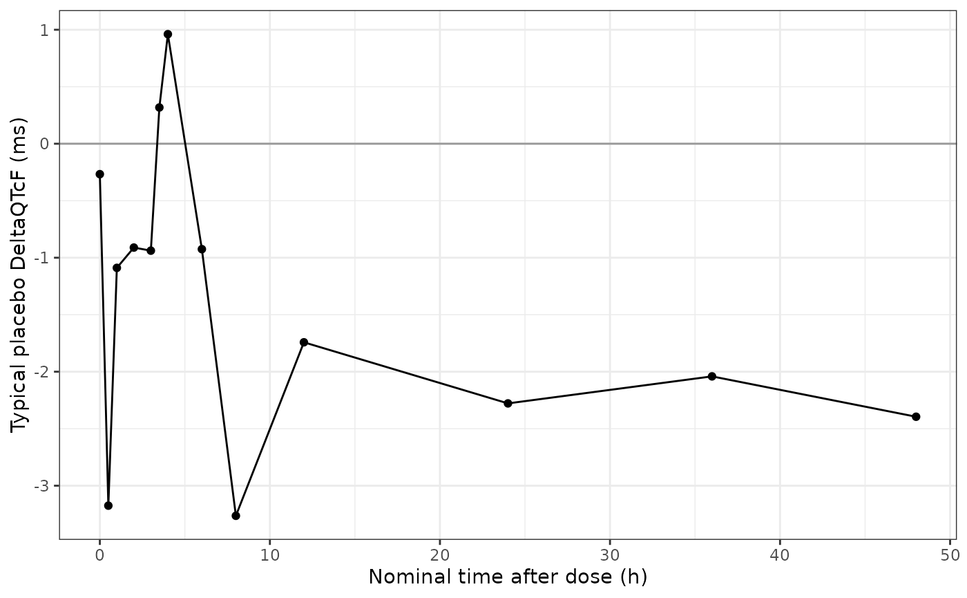
Typical placebo DeltaQTcF over the nominal dECG times. Compare the placebo (yellow) line of the bottom panel of Figure 1 of Sundell 2025: a dip at 0.5 h and 8 h, a peak at 4 h, and values about 2 ms below baseline from 24 h onwards.
Placebo-corrected effect at the clinical and supratherapeutic exposures (Table 1)
Table 1 of Sundell 2025 reports the model-predicted mean
placebo-corrected effect at the high clinical exposure scenario (2.16
umol/L: the steady-state Cmax of 40 mg once daily as capsules, fed, with
a strong CYP3A4 inhibitor) and at the highest observed concentration
(16.70 umol/L, 1200 mg fractionated). The model reproduces it as an
active-arm prediction at concentration C minus a placebo
prediction at zero concentration, at the same nominal time and baseline.
The contrast is evaluated at every nominal time and at off-centre
baselines, because all other terms must cancel.
conc_tab1 <- c(2.16, 16.70)
tab1 <- data.frame(
  Exposure = c("High clinical exposure (40 mg)", "Supratherapeutic (1200 mg fractionated)"),
  conc = conc_tab1,
  published = c(0.35, 0.31),
  model = ddelta(mod_typ, conc_tab1)
) |>
  dplyr::mutate(pct_diff = 100 * (model - published) / published)

grid <- expand.grid(ntime = ntime_levels, qtc_bl = c(380, 420))
spread <- vapply(seq_len(nrow(grid)), function(i) {
  max(abs(ddelta(mod_typ, conc_tab1, grid$ntime[i], grid$qtc_bl[i]) - tab1$model))
}, numeric(1))

stopifnot(
  max(spread) < 1e-10,
  # Exact identity with the closed form theta1 + theta2 * C
  isTRUE(all.equal(tab1$model, 0.359 - 0.003 * conc_tab1, tolerance = 1e-12)),
  # Against the published means; the gap is the rounding of the printed values.
  all(abs(tab1$pct_diff) < 3)
)

tab1 |>
  dplyr::rename(
    "Balcinrenone exposure" = Exposure,
    "Cmax (umol/L)" = conc,
    "DeltaDeltaQTcF published (ms)" = published,
    "DeltaDeltaQTcF model (ms)" = model,
    "% diff" = pct_diff
  ) |>
knitr::kable(digits = 3, caption = "Replicates Table 1 of Sundell 2025 (mean placebo-corrected effects, primary analysis).")| Balcinrenone exposure | Cmax (umol/L) | DeltaDeltaQTcF published (ms) | DeltaDeltaQTcF model (ms) | % diff |
|---|---|---|---|---|
| High clinical exposure (40 mg) | 2.16 | 0.35 | 0.353 | 0.720 |
| Supratherapeutic (1200 mg fractionated) | 16.70 | 0.31 | 0.309 | -0.355 |
The model reproduces both published means to within 1%. The 90% confidence intervals of Table 1 cannot be reproduced, because they depend on the sampling covariance of theta1 and theta2, which is not reported.
conc_grid <- seq(0, 16.7, by = 0.1)
curve_df <- data.frame(conc = conc_grid, value = ddelta(mod_typ, conc_grid))
ggplot(curve_df, aes(conc, value)) +
  geom_line() +
  geom_vline(xintercept = 2.156, linetype = "dashed", colour = "steelblue") +
  geom_hline(yintercept = 10, linetype = "dotted", colour = "firebrick") +
  coord_cartesian(ylim = c(-5, 12)) +
  labs(x = "Balcinrenone concentration (umol/L)", y = "DeltaDeltaQTcF (ms)") +
  theme_bw()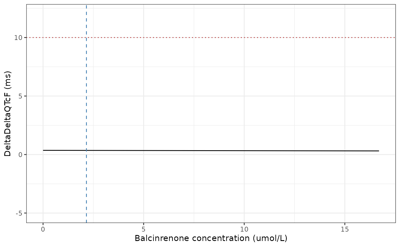
Typical placebo-corrected effect over the observed concentration range. Replicates the mean line of Figure 4 of Sundell 2025; the dashed vertical line is the 2.156 umol/L high clinical exposure scenario and the dotted horizontal line the 10 ms threshold of regulatory concern.
Sensitivity analysis excluding the 1200 mg arm (Table S2)
Because heart rate rose by a mean 10.2 bpm after the 1200 mg fractionated dose, the authors refitted the same model without that arm (Table S1, lower block). The refit is not packaged as a separate model; its estimates are substituted into the packaged structure here to check Table S2.
mod_sens <- rxode2::ini(
  mod_typ,
  e0 = -0.377, e_on_treatment_e0 = 0.479, slope = -0.140,
  e_ntime0p5_e0 = -2.472, e_ntime1_e0 = -0.401, e_ntime2_e0 = -0.333,
  e_ntime3_e0 = -0.429, e_ntime3p5_e0 = 0.667, e_ntime4_e0 = 1.260,
  e_ntime6_e0 = -0.924, e_ntime8_e0 = -2.679, e_ntime12_e0 = -1.090,
  e_ntime24_e0 = -2.287, e_ntime36_e0 = -1.642, e_ntime48_e0 = -2.224,
  e_qtc_bl_e0 = -0.047
)
#> ℹ change initial estimate of `e0` to `-0.377`
#> ℹ change initial estimate of `e_on_treatment_e0` to `0.479`
#> ℹ change initial estimate of `slope` to `-0.14`
#> ℹ change initial estimate of `e_ntime0p5_e0` to `-2.472`
#> ℹ change initial estimate of `e_ntime1_e0` to `-0.401`
#> ℹ change initial estimate of `e_ntime2_e0` to `-0.333`
#> ℹ change initial estimate of `e_ntime3_e0` to `-0.429`
#> ℹ change initial estimate of `e_ntime3p5_e0` to `0.667`
#> ℹ change initial estimate of `e_ntime4_e0` to `1.26`
#> ℹ change initial estimate of `e_ntime6_e0` to `-0.924`
#> ℹ change initial estimate of `e_ntime8_e0` to `-2.679`
#> ℹ change initial estimate of `e_ntime12_e0` to `-1.09`
#> ℹ change initial estimate of `e_ntime24_e0` to `-2.287`
#> ℹ change initial estimate of `e_ntime36_e0` to `-1.642`
#> ℹ change initial estimate of `e_ntime48_e0` to `-2.224`
#> ℹ change initial estimate of `e_qtc_bl_e0` to `-0.047`
conc_s2 <- c(2.16, 14.30)
tab_s2 <- data.frame(
  Exposure = c("High clinical exposure (40 mg)", "Supratherapeutic (800 mg fractionated)"),
  conc = conc_s2,
  published = c(0.18, -1.53),
  model = ddelta(mod_sens, conc_s2)
) |>
  dplyr::mutate(pct_diff = 100 * (model - published) / published)

stopifnot(
  isTRUE(all.equal(tab_s2$model, 0.479 - 0.140 * conc_s2, tolerance = 1e-12)),
  all(abs(tab_s2$pct_diff) < 3)
)

tab_s2 |>
  dplyr::rename(
    "Balcinrenone exposure" = Exposure,
    "Cmax (umol/L)" = conc,
    "DeltaDeltaQTcF published (ms)" = published,
    "DeltaDeltaQTcF model (ms)" = model,
    "% diff" = pct_diff
  ) |>
knitr::kable(digits = 3, caption = "Replicates Table S2 of Sundell 2025 (sensitivity analysis without the 1200 mg fractionated arm).")| Balcinrenone exposure | Cmax (umol/L) | DeltaDeltaQTcF published (ms) | DeltaDeltaQTcF model (ms) | % diff |
|---|---|---|---|---|
| High clinical exposure (40 mg) | 2.16 | 0.18 | 0.177 | -1.889 |
| Supratherapeutic (800 mg fractionated) | 14.30 | -1.53 | -1.523 | -0.458 |
Driving the model from a dose
The QTc model needs a balcinrenone concentration at each ECG time.
Here the concentrations come from
Parkinson_2025_balcinrenone, for the dosing behind the high
clinical exposure scenario: 40 mg once daily as capsules, fed, in
healthy phase 1 participants. The PK model returns nmol/L, so its output
is divided by 1000. Body weight and eGFR are drawn from the phase 1
distributions used in the Parkinson 2025 vignette (83.8 (15.1) kg; 96.2
(12.8) mL/min/1.73 m^2). The strong CYP3A4 inhibitor is not part of the
PK model; the paper applies it as a 2.22-fold increase in Cmax
(Discussion), so the scenario’s Cmax without the inhibitor is 2.156 /
2.22 = 0.971 umol/L.
n_sub <- 100L
tau <- 24
n_dose <- 10L
mw_balcinrenone <- 399.4 # g/mol (PubChem CID 118599727)
ss_start <- (n_dose - 1L) * tau

set.seed(20250205)
subj <- data.frame(
  id = seq_len(n_sub),
  WT = pmin(pmax(rnorm(n_sub, 83.8, 15.1), 50), 100),
  CRCL = pmin(pmax(rnorm(n_sub, 96.2, 12.8), 76.7), 115),
  FED = 1, STUDY_BALCINRENONE_PHASE1 = 1, DOSE_BALCINRENONE_MG = 40
)
dose_rows <- merge(subj, data.frame(time = tau * (seq_len(n_dose) - 1L)), by = NULL) |>
  # rate = -2: the model's dur(depot) sets the zero-order absorption window.
  dplyr::mutate(evid = 1L, amt = 40 * 1e6 / mw_balcinrenone, cmt = "depot", rate = -2)
obs_rows <- merge(subj, data.frame(time = ss_start + seq(0, tau, by = 0.25)), by = NULL) |>
  dplyr::mutate(evid = 0L, amt = NA_real_, cmt = "central", rate = NA_real_)
pk_events <- dplyr::bind_rows(dose_rows, obs_rows) |>
  dplyr::arrange(id, time, dplyr::desc(evid))

pk_sim <- as.data.frame(rxode2::rxSolve(
  readModelDb("Parkinson_2025_balcinrenone"), events = pk_events,
  returnType = "data.frame"
)) |>
  dplyr::filter(time >= ss_start) |>
  dplyr::transmute(
    id, time = time - ss_start, conc_um = Cc / 1000,
    treatment = "40 mg QD fed"
  )
PKNCA on the driving concentrations
conc_obj <- PKNCA::PKNCAconc(
  pk_sim |> dplyr::filter(!is.na(conc_um)),
  conc_um ~ time | treatment + id
)
dose_obj <- PKNCA::PKNCAdose(
  data.frame(id = seq_len(n_sub), time = 0, amt = 40, treatment = "40 mg QD fed"),
  amt ~ time | treatment + id
)
intervals <- data.frame(start = 0, end = tau, cmax = TRUE, tmax = TRUE, auclast = TRUE)
nca_res <- PKNCA::pk.nca(PKNCA::PKNCAdata(conc_obj, dose_obj, intervals = intervals))

cmp <- nlmixr2lib::ncaComparisonTable(
  simulated = nca_res,
  reference = data.frame(treatment = "40 mg QD fed", cmax = 2.156 / 2.22),
  by = "treatment",
  units = c(cmax = "umol/L"),
  tolerance_pct = 20
)
knitr::kable(cmp, caption = "Simulated steady-state Cmax (median) against the high clinical exposure scenario without the 2.22-fold CYP3A4-inhibitor factor (2.156 / 2.22 umol/L).")| NCA parameter | treatment | Reference | Simulated | % diff |
|---|---|---|---|---|
| Cmax (umol/L) | 40 mg QD fed | 0.971 | 0.96 | -1.1% |
nca_summary <- as.data.frame(nca_res$result) |>
  dplyr::filter(PPTESTCD %in% c("cmax", "tmax", "auclast")) |>
  dplyr::group_by(PPTESTCD) |>
  dplyr::summarise(
    median = stats::median(PPORRES),
    p05 = stats::quantile(PPORRES, 0.05),
    p95 = stats::quantile(PPORRES, 0.95),
    .groups = "drop"
  ) |>
  dplyr::rename(
    "NCA parameter" = PPTESTCD,
    "Median" = median,
    "5th percentile" = p05,
    "95th percentile" = p95
  )
knitr::kable(nca_summary, digits = 3, caption = "NCA of the simulated steady-state dosing interval (umol/L, h).")| NCA parameter | Median | 5th percentile | 95th percentile |
|---|---|---|---|
| auclast | 4.059 | 2.327 | 7.816 |
| cmax | 0.960 | 0.466 | 1.924 |
| tmax | 2.000 | 0.750 | 6.775 |
Sundell 2025 does not report NCA; the only exposure it gives for the therapeutic dose is the 2.156 umol/L scenario, itself derived from another study (NCT04798222) and an inhibitor factor that are not in the paper. The comparison is therefore a plausibility check of the PK driver, not a test of the QTc model, which was fitted to observed concentrations.
Placebo-corrected effect along the profile
The placebo-corrected effect at each simulated concentration, with the inhibitor factor applied to the concentration, stays within a fraction of a millisecond of theta1 because the slope is essentially zero.
prof <- pk_sim |>
  dplyr::mutate(conc_inh = 2.22 * conc_um)
prof$ddqtcf <- ddelta(mod_typ, prof$conc_inh)

stopifnot(
  # Exact identity per row: theta1 + theta2 * C
  isTRUE(all.equal(prof$ddqtcf, 0.359 - 0.003 * prof$conc_inh, tolerance = 1e-12))
)

prof |>
  dplyr::group_by(time) |>
  dplyr::summarise(
    med = stats::median(ddqtcf),
    lo = stats::quantile(ddqtcf, 0.05),
    hi = stats::quantile(ddqtcf, 0.95),
    .groups = "drop"
  ) |>
  ggplot(aes(time, med)) +
  geom_ribbon(aes(ymin = lo, ymax = hi), alpha = 0.3) +
  geom_line() +
  labs(x = "Time after the last dose (h)", y = "DeltaDeltaQTcF (ms)") +
  theme_bw()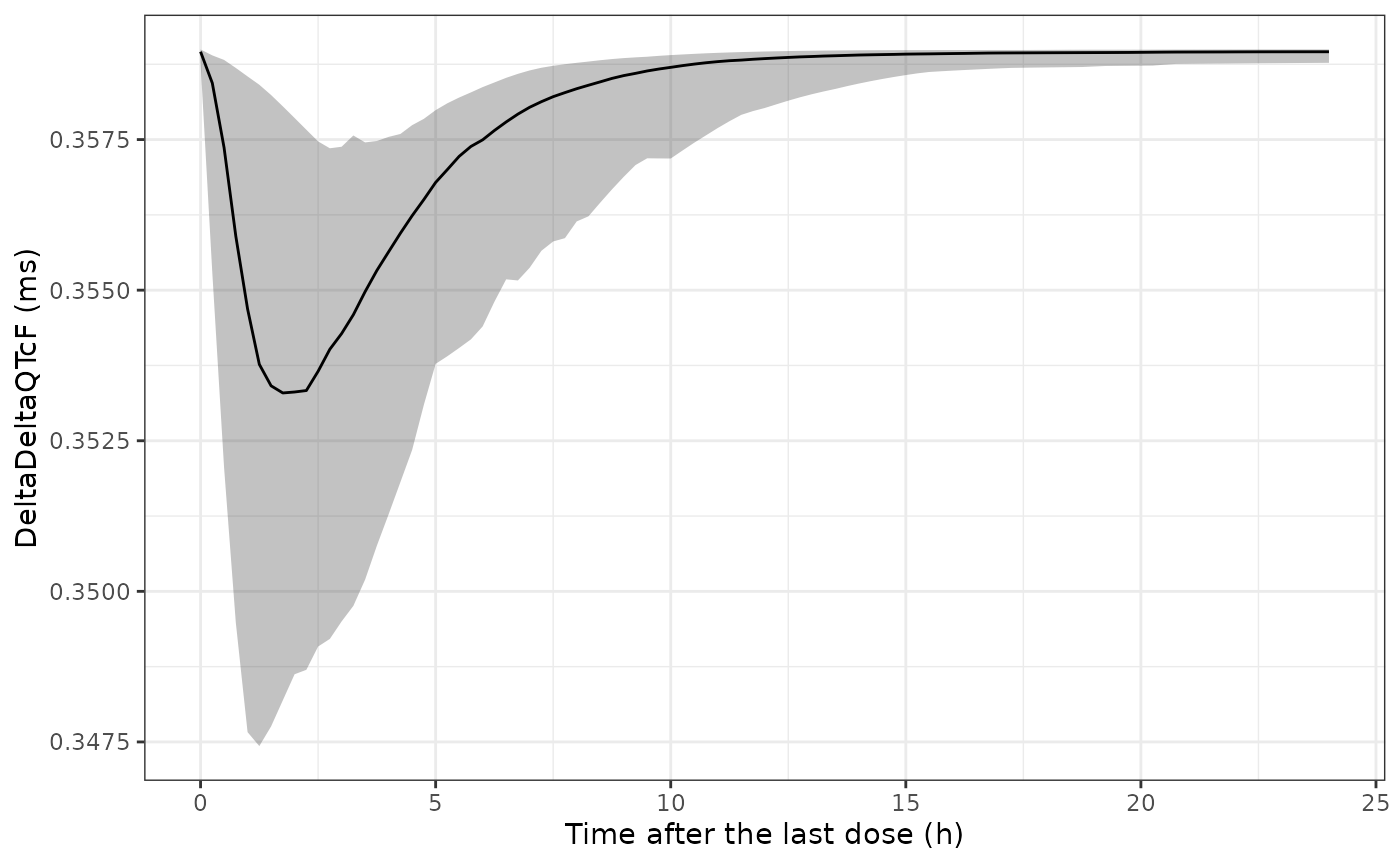
Typical DeltaDeltaQTcF over the simulated steady-state dosing interval (median and 5th-95th percentile across subjects), with the 2.22-fold CYP3A4-inhibitor factor applied to concentration.
Assumptions and deviations
- Random effects and residual error not reported. Equation 1 has random effects on the intercept and the slope with an unstructured covariance, and the lme4 fit has a residual error, but the paper and its supplements report only the fixed effects (Table S1). The two random effects and the residual SD are therefore fixed to zero. The packaged model gives typical-value predictions only; it cannot reproduce the spread of Figure 2 or the confidence intervals of Tables 1 and S2.
- Centering constant. The model centres baseline QTcF on the overall mean of all baseline values, which the paper does not print, and no baseline QTcF summary is reported. The rounded 400 ms is used. An error of d ms in this constant shifts every DeltaQTcF prediction by 0.052 d ms and cancels exactly in DeltaDeltaQTcF.
-
Nominal-time reference. Table S1 lists ‘Time = 0’
(pre-dose) as the reference level.
NTIMEis binned to the nearest scheduled level inside the model, so a value between grid points is assigned to the closest one. The 3.5 h level was sampled only in the 800 and 1200 mg fractionated arms. -
Treatment indicator. The lme4 code enters treatment
as a factor (
TRTID), but Table S1 reports one active-arm coefficient against placebo, so all dose groups share one treatment intercept (ON_TREATMENT= 1). - Sensitivity analysis. The refit without the 1200 mg arm is reproduced above by substituting its Table S1 estimates, not packaged as a separate model. The Discussion quotes a sensitivity-analysis DeltaDeltaQTcF of -0.66 ms (90% CI -2.73, 1.42) without naming the concentration; it matches neither row of Table S2 (0.18 ms at 2.16 umol/L, -1.53 ms at 14.30 umol/L) and corresponds to about 8.1 umol/L under the refit estimates. Table S2 is used as the reference.
-
Upstream PK. The concentration driver is the
separately published
Parkinson_2025_balcinrenonemodel, fitted to capsule data; the QTc study used an oral suspension, and the QTc model was fitted to observed concentrations. The phase 1 covariate distributions and the 2.22-fold CYP3A4-inhibitor factor applied to concentration are assumptions of this vignette. - Molar mass. 399.4 g/mol (PubChem CID 118599727) is used to convert the 40 mg dose to nmol for the PK model; it is not reported in Sundell 2025.