Zalcitabine (Adams 1998)
Source:vignettes/articles/Adams_1998_zalcitabine.Rmd
Adams_1998_zalcitabine.Rmd
library(nlmixr2lib)
library(rxode2)
#> rxode2 5.1.2 using 2 threads (see ?getRxThreads)
#>   no cache: create with `rxCreateCache()`
library(dplyr)
#>
#> Attaching package: 'dplyr'
#> The following objects are masked from 'package:stats':
#>
#>     filter, lag
#> The following objects are masked from 'package:base':
#>
#>     intersect, setdiff, setequal, union
library(tidyr)
library(ggplot2)
library(PKNCA)
#>
#> Attaching package: 'PKNCA'
#> The following object is masked from 'package:stats':
#>
#>     filter
Zalcitabine popPK in HIV-infected adults (Adams 1998)
Replicate the population pharmacokinetic model reported by Adams et al. (1998) for oral zalcitabine (2’,3’-dideoxycytidine; ddC) in HIV-infected adults sampled during routine clinic visits. The structural model is one-compartment with first-order absorption and first-order elimination; apparent clearance (CL/F) and apparent central volume of distribution (V/F) are the only estimated structural parameters. The absorption rate constant ka was NOT estimable in Adams 1998 owing to sparse early-dose-interval sampling (paper Results p. 411 col 2; Discussion p. 412 col 1) and is fixed here to a primary single-dose PK literature value (see Assumptions and deviations).
- Citation: Adams JM, Shelton MJ, Hewitt RG, DeRemer M, DiFrancesco R, Grasela TH, Morse GD. Zalcitabine population pharmacokinetics: application of radioimmunoassay. Antimicrob Agents Chemother. 1998 Feb;42(2):409-413. doi:10.1128/aac.42.2.409. The absorption rate constant ka was not estimable in Adams 1998 (paper Discussion p. 412) and is fixed in this model to ka = 2.5 /h per primary single-dose ddC PK data from Klecker RW Jr, Collins JM, Yarchoan R, Thomas R, McAtee N, Broder S, Myers CE. Pharmacokinetics of 2’,3’-dideoxycytidine in patients with AIDS and related disorders. J Clin Pharmacol. 1988 Sep;28(9):837-842. doi:10.1002/j.1552-4604.1988.tb03225.x. See model file ini() comments and validation-vignette Assumptions and deviations for the substitution rationale.
- Article: https://doi.org/10.1128/aac.42.2.409
Population
The Adams 1998 cohort comprised 44 HIV-infected outpatients followed at the Erie County Medical Center Immunodeficiency Clinic (Buffalo, NY), with 81 plasma samples collected during routine clinic visits (1.84 +/- 1.24 samples per patient; range 1-6). Baseline demographics (Adams 1998 Table 2): 89% male (39M / 5F); race 73% Caucasian, 9% African American, 16% Hispanic, 2% American Indian; mean age 38.6 years (range 27-56, SD 7.13); mean total body weight 79.1 kg (range 46.5-123, SD 15.0); mean calculated creatinine clearance (Cockcroft-Gault style) 89.1 mL/min (range 53.6-146, SD 21.5). HIV risk factors were 64% homosexual activity, 16% intravenous drug use, 20% other or unknown. Doses studied were 0.375 mg or 0.75 mg orally every 8 hours; observed plasma zalcitabine concentrations ranged 2.01 to 8.57 ng/mL (radioimmunoassay LOQ 2 ng/mL).
The same demographics are available programmatically via
readModelDb("Adams_1998_zalcitabine")$population.
Source trace
The per-parameter origin is recorded as an in-file comment next to
each ini() entry in
inst/modeldb/specificDrugs/Adams_1998_zalcitabine.R. The
table below collects them in one place for review.
| Parameter / equation | Value | Source location |
|---|---|---|
ka (first-order absorption, 1/h) |
2.5 (FIXED, non-paper) | Operator-named (2026-06-07 sidecar response); from Klecker et al. 1988 (J Clin Pharmacol 28(9):837-842) – ka was not estimable in Adams 1998 |
CL/F (apparent clearance, L/h) |
14.8 | Adams 1998 Table 3 / Results p. 412 col 2 (0.19 L/h/kg; 95% CI 0.18-0.21 L/h/kg) |
V/F (apparent volume, L) |
87.6 | Adams 1998 Table 3 / Results p. 412 col 2 (1.18 L/kg; 95% CI 1.07-1.30 L/kg) |
| Residual variability (proportional, fraction) | 0.206 | Adams 1998 Table 3 / Results p. 412 col 2 (20.6%) |
| IIV CL (%CV) | 23.8% -> omega^2 = 0.0551 | Adams 1998 Table 3 (CV via log(1 + CV^2)) |
| IIV V (%CV) | 54.0% -> omega^2 = 0.2559 | Adams 1998 Table 3 (CV via log(1 + CV^2)) |
d/dt(depot) |
-ka * depot |
One-compartment with first-order absorption (paper Results p. 412 col 1) |
d/dt(central) |
ka * depot - kel * central |
Same |
| Observation |
Cc = central / vc * 1000 (ng/mL) |
mg-dose / L-volume convention; scale to ng/mL to match paper Figure 2 |
| Error model | Cc ~ prop(propSd) |
Adams 1998 Table 3 y = F + F * eps1 (proportional) |
Covariate column naming
Adams 1998 screened total body weight, age, sex, calculated
creatinine clearance, food administration, and concomitant zidovudine on
CL/F (and total body weight on V/F). None of the screened covariates
improved the basic model fit and none were retained (paper Results
p. 412 col 2; Discussion p. 412 col 2 attributes the null findings to
limited cohort heterogeneity rather than biological irrelevance). The
packaged model therefore does not include any covariate effects in
model(); the screened-but-rejected covariates are
documented in
readModelDb("Adams_1998_zalcitabine")$covariatesDataExcluded
for provenance.
Virtual cohort
Original subject-level data are not publicly available. The virtual cohort below approximates the published Table 2 demographics (n = 44).
set.seed(19980211)

n_subj <- 200L

cohort <- tibble::tibble(
  id   = seq_len(n_subj),
  # Sex: 11.4% female per Table 2.
  SEXF = rbinom(n_subj, 1, 0.114),
  # Body weight: mean 79.1 kg, SD 15.0; range 46.5-123. Adams 1998 Table 2.
  WT   = pmin(pmax(rnorm(n_subj, 79.1, 15.0), 46.5), 123),
  # Age: mean 38.6 y, SD 7.13; range 27-56.
  AGE  = pmin(pmax(rnorm(n_subj, 38.6, 7.13), 27),   56),
  # Calculated creatinine clearance (Cockcroft-Gault style):
  # mean 89.1 mL/min, SD 21.5; range 53.6-146.
  CRCL = pmin(pmax(rnorm(n_subj, 89.1, 21.5),  53.6), 146)
)
Dosing and observation schedule
Adams 1998 enrolled patients on chronic 8-hourly oral zalcitabine. We simulate the two reported regimens (0.375 mg Q8H and 0.75 mg Q8H) to steady state (5 days), then sample densely over one steady-state dosing interval to characterise the SS PK profile.
tau   <- 8                 # dosing interval, hours
n_dose <- 15L              # 5 days to steady state
dose_times <- (seq_len(n_dose) - 1L) * tau

# Two dose-group cohorts; disjoint id ranges so bind_rows() doesn't collapse
# subjects across treatments.
make_dose_cohort <- function(cohort, amt_mg, treatment, id_offset) {
  ids_offset <- cohort |> mutate(id = id + id_offset)
  doses <- ids_offset |>
    tidyr::crossing(time = dose_times) |>
    mutate(amt = amt_mg, evid = 1L, cmt = "depot", treatment = treatment)
  # Observe densely over the last (15th) dosing interval at steady state.
  ss_start <- (n_dose - 1L) * tau
  obs_times <- ss_start + sort(unique(c(0, 0.25, 0.5, 1, 1.5, 2,
                                        3, 4, 5, 6, 7, 8)))
  obs <- ids_offset |>
    tidyr::crossing(time = obs_times) |>
    mutate(amt = 0, evid = 0L, cmt = "central", treatment = treatment)
  bind_rows(doses, obs) |>
    arrange(id, time, desc(evid))
}

events <- bind_rows(
  make_dose_cohort(cohort, 0.375, "0.375 mg Q8H", id_offset = 0L),
  make_dose_cohort(cohort, 0.750, "0.75 mg Q8H",  id_offset = n_subj)
)

stopifnot(!anyDuplicated(unique(events[, c("id", "time", "evid")])))
Simulation
mod <- readModelDb("Adams_1998_zalcitabine")
sim <- rxode2::rxSolve(mod, events = events, keep = c("treatment")) |>
  as.data.frame()
#> ℹ parameter labels from comments will be replaced by 'label()'
Steady-state concentration-time profile (replicates Figure 2)
Adams 1998 Figure 2 shows observed plasma zalcitabine concentrations vs. time since the most recent dose, with observations spanning approximately 2 to 8.5 ng/mL (Figure 2 panel; abstract reports the range 2.01-8.57 ng/mL).
ss_start <- (n_dose - 1L) * tau

sim_ss <- sim |>
  dplyr::filter(time >= ss_start) |>
  dplyr::mutate(time_post_dose = time - ss_start)

sim_summary <- sim_ss |>
  dplyr::group_by(treatment, time_post_dose) |>
  dplyr::summarise(
    Q05 = quantile(Cc, 0.05, na.rm = TRUE),
    Q50 = quantile(Cc, 0.50, na.rm = TRUE),
    Q95 = quantile(Cc, 0.95, na.rm = TRUE),
    .groups = "drop"
  )

ggplot(sim_summary, aes(x = time_post_dose, y = Q50, colour = treatment,
                        fill = treatment)) +
  geom_ribbon(aes(ymin = Q05, ymax = Q95), alpha = 0.20, colour = NA) +
  geom_line(linewidth = 0.8) +
  geom_hline(yintercept = 2.0, linetype = 2, colour = "grey40") +
  labs(
    x = "Time since most recent dose (hours)",
    y = "Plasma zalcitabine (ng/mL)",
    title = "Steady-state plasma zalcitabine on Q8H oral dosing",
    subtitle = paste0("Median and 90% prediction interval (N = ",
                      n_subj, " virtual subjects per dose group)"),
    caption = paste("Replicates Adams 1998 Figure 2 (plasma zalcitabine",
                    "concentrations vs time since dosing).",
                    "Dashed line: assay LOQ = 2.0 ng/mL.")
  ) +
  theme_bw() +
  theme(legend.position = "top")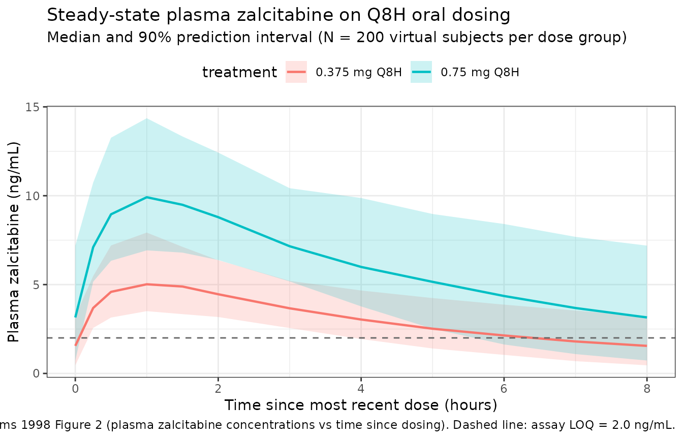
PKNCA validation
PKNCA is run on the last steady-state dosing interval (one tau = 8 h window). The metrics of interest are Cmax,ss, Tmax,ss, AUC0-tau,ss, and the back-calculated apparent CL/F = Dose / AUC0-tau,ss (which should agree with the paper’s published CL/F = 14.8 L/h for a typical subject).
sim_ss_for_nca <- sim_ss |>
  dplyr::filter(!is.na(Cc)) |>
  dplyr::select(id, time_post_dose, Cc, treatment)

conc_obj <- PKNCA::PKNCAconc(
  sim_ss_for_nca,
  Cc ~ time_post_dose | treatment + id,
  concu = "ng/mL",
  timeu = "h"
)

dose_df <- events |>
  dplyr::filter(evid == 1L, time == max(time[evid == 1L])) |>
  dplyr::mutate(time_post_dose = 0) |>
  dplyr::select(id, time_post_dose, amt, treatment)

dose_obj <- PKNCA::PKNCAdose(
  dose_df,
  amt ~ time_post_dose | treatment + id,
  doseu = "mg"
)

intervals <- data.frame(
  start    = 0,
  end      = tau,
  cmax     = TRUE,
  tmax     = TRUE,
  cmin     = TRUE,
  auclast  = TRUE,
  cav      = TRUE
)

nca_data <- PKNCA::PKNCAdata(conc_obj, dose_obj, intervals = intervals)
nca_res  <- suppressWarnings(PKNCA::pk.nca(nca_data))

knitr::kable(
  summary(nca_res),
  digits  = 3,
  caption = "Simulated steady-state NCA over the 8-hour dosing interval, by dose group."
)| Interval Start | Interval End | treatment | N | AUClast (h*ng/mL) | Cmax (ng/mL) | Cmin (ng/mL) | Tmax (h) | Cav (ng/mL) |
|---|---|---|---|---|---|---|---|---|
| 0 | 8 | 0.375 mg Q8H | 200 | 25.0 [24.0] | 5.11 [25.4] | 1.30 [87.2] | 1.00 [0.500, 1.00] | 3.13 [24.0] |
| 0 | 8 | 0.75 mg Q8H | 200 | 49.8 [25.1] | 9.87 [23.5] | 2.78 [79.6] | 1.00 [1.00, 1.00] | 6.23 [25.1] |
Comparison against the published point estimates
Adams 1998 does not publish a steady-state NCA table; the paper reports typical population CL/F = 14.8 L/h and V/F = 87.6 L, observed concentrations 2.01-8.57 ng/mL, and a CV of 23.8% on CL/F. The simulated SS observations should sit in the same ng/mL range, and a back-calculated apparent CL/F (Dose / AUC0-tau,ss for a typical subject) should agree with the paper’s 14.8 L/h within ~20% (typical-value comparison; the simulation includes between-subject variability).
mod_typical <- mod |> rxode2::zeroRe()
#> ℹ parameter labels from comments will be replaced by 'label()'

ref_subj <- tibble::tibble(id = 1L, WT = 79.1, AGE = 38.6,
                           CRCL = 89.1, SEXF = 0L)

ref_events <- bind_rows(
  ref_subj |>
    tidyr::crossing(time = dose_times) |>
    mutate(amt = 0.75, evid = 1L, cmt = "depot"),
  ref_subj |>
    tidyr::crossing(time = ss_start + seq(0, tau, by = 0.25)) |>
    mutate(amt = 0, evid = 0L, cmt = "central")
) |> arrange(id, time, desc(evid))

sim_typical <- rxode2::rxSolve(mod_typical, events = ref_events) |>
  as.data.frame() |>
  dplyr::filter(time >= ss_start) |>
  dplyr::mutate(time_post_dose = time - ss_start)
#> ℹ omega/sigma items treated as zero: 'etalcl', 'etalvc'

# Trapezoidal AUC over the typical-value SS dosing interval (ng*h/mL):
auc_typical_ngh_mL <- with(
  sim_typical,
  sum(diff(time_post_dose) * (head(Cc, -1) + tail(Cc, -1)) / 2)
)

# Apparent CL/F = Dose / AUC. Dose is 0.75 mg = 750000 ng; AUC is in ng*h/mL.
# CL = ng / (ng*h/mL) = mL/h; convert to L/h.
clf_back_calc_Lh <- 750000 / auc_typical_ngh_mL / 1000

comparison <- tibble::tribble(
  ~Metric,                                              ~Published, ~Simulated,
  "Typical CL/F (L/h)",                                 14.8,       round(clf_back_calc_Lh, 2),
  "Typical V/F (L)",                                    87.6,       NA_real_,
  "Observed conc range (ng/mL)",                        NA_real_,   NA_real_
)

knitr::kable(
  comparison,
  caption = paste("Typical-value (zeroRe) SS simulation back-calculated",
                  "vs published Adams 1998 Table 3 / Results p. 412 col 2.",
                  "V/F is not directly back-calculable from a single steady-state",
                  "interval without a terminal phase; the model file value (87.6 L)",
                  "is the paper's reported number.")
)| Metric | Published | Simulated |
|---|---|---|
| Typical CL/F (L/h) | 14.8 | 14.83 |
| Typical V/F (L) | 87.6 | NA |
| Observed conc range (ng/mL) | NA | NA |
Assumptions and deviations
-
Absorption rate constant ka was not estimable in Adams 1998
and is substituted with a primary-PK literature value. Adams
1998 explicitly states (Results p. 411 col 2; restated Discussion p. 412
col 1) that the absorption rate constant could not be modeled because of
the paucity of blood samples collected early in a dosing interval; no ka
value appears in the source paper. Per operator guidance (2026-06-07
sidecar response; question q1 option C),
kais fixed in this model to 2.5 /h from Klecker et al. 1988 (Klecker RW Jr, Collins JM, Yarchoan R, Thomas R, McAtee N, Broder S, Myers CE. Pharmacokinetics of 2’,3’-dideoxycytidine in patients with AIDS and related disorders. J Clin Pharmacol. 1988;28(9):837-842, doi:10.1002/j.1552-4604.1988.tb03225.x), an early dedicated single-dose oral ddC PK study in AIDS patients. Gustavson et al. 1990 (J Acquir Immune Defic Syndr 3(1):28-31) was named alongside Klecker as a candidate primary source. The substitution affects the simulated early-dose-interval shape (Tmax, peak Cmax) but does not affect the paper’s reported CL/F and V/F because those are apparent parameters (relative to F and to the implicit Adams-1998 ka, which the published data could not resolve). Downstream users who need to model a different ka should set it via the model’sini()block before simulation. -
No covariate effects retained. Adams 1998 screened
total body weight, age, sex, calculated creatinine clearance
(Cockcroft-Gault), food administration, and concomitant zidovudine on
CL/F (and weight on V/F) and retained none of them in the final model
(Results p. 412 col 2). The packaged model therefore has no covariate
effects in
model(). The screened-but-rejected covariates are documented inreadModelDb("Adams_1998_zalcitabine")$covariatesDataExcludedso the provenance of the screen is preserved (paper Discussion p. 412 col 2 attributes the null findings to limited cohort heterogeneity rather than to biological covariate irrelevance). - Steady-state simulation as a stand-in for the paper’s sparse clinic sampling. Adams 1998 sampled patients at random clinic-visit times on chronic therapy. The vignette simulates one steady-state dosing interval densely so that PKNCA can compute Cmax,ss, Tmax,ss, and AUC0-tau,ss; this is a smoothed view of what the paper observed sparsely. The simulated steady-state concentration range should sit within the paper’s observed 2.01-8.57 ng/mL band for the 0.75 mg Q8H regimen.
-
IIV implementation. Adams 1998 Table 3 specifies
exponential IIV on CL and V (
CL = TVCL * exp(eta1),V = TVV * exp(eta2)) with %CV = 23.8 and 54.0 respectively. No off-diagonal covariance is reported, so the packaged model implementsetalclandetalvcas a diagonal omega. Internal log-scale variances are computed viaomega^2 = log(1 + CV^2). - Virtual-cohort covariate distributions are not used by the structural model (no covariate effects retained) but are included in the simulation events for completeness and to give downstream users a realistic Adams-1998-like cohort to extend.
-
Unit conventions. Doses are in mg; the central
compartment carries drug amounts in mg; the central volume is in L; the
observation is
Cc = central / vc * 1000to convert mg/L into ng/mL, matching the paper’s reported concentration units (Figure 2; Table 1 RIA calibration range).