Isavuconazole (Martin-Cerezuela 2024)
Source:vignettes/articles/MartinCerezuela_2024_isavuconazole.Rmd
MartinCerezuela_2024_isavuconazole.RmdModel and source
- Citation: Martin-Cerezuela M, Maya Gallegos C, Marques-Minana MR, Broch Porcar MJ, Cruz-Sanchez A, Mateo-Pardo JC, Peris Ribera JE, Gimeno R, Castellanos-Ortega A, Poveda Andres JL, Ramirez Galleymore P, Lipman J, Di Paolo A, Breilh D. Isavuconazole Pharmacokinetics in Critically Ill Patients: Relationship with Clinical Effectiveness and Patient Safety. Antibiotics (Basel). 2024;13(8):706. doi:10.3390/antibiotics13080706. PMCID PMC11350865.
- Description: One-compartment population PK model for intravenous isavuconazole (dosed as the prodrug isavuconazonium sulfate, doses expressed as isavuconazole) in critically ill adults in a medical intensive care unit, a third of them on continuous renal replacement therapy and a third on extracorporeal membrane oxygenation, with a 1-h infusion into the central compartment and first-order elimination (Martin-Cerezuela 2024). No covariates were retained. The residual error model is not reported and is carried as zero.
- Article: https://doi.org/10.3390/antibiotics13080706 (PMC11350865; open access, CC BY)
- Preprint: https://doi.org/10.21203/rs.3.rs-4027011/v1 (Research Square)
Martin-Cerezuela and colleagues followed 24 critically ill adults in a Spanish medical intensive care unit who received intravenous isavuconazole at the labelled regimen. They drew three plasma samples per patient (predose, 1 h and 12 h after the infusion) after 48-96 h of treatment and fitted a population PK model in NONMEM (ADVAN1 TRANS2, FOCE with interaction). A one-compartment model with first-order elimination described the 71 concentrations. None of the screened covariates – including continuous renal replacement therapy (CRRT) and extracorporeal membrane oxygenation (ECMO) – improved the model, so the final model has none.
No erratum or correction was found in Europe PMC or on the journal landing page (checked 2026-10-30).
Population
data.frame(
  Characteristic = c(
    "Patients / plasma concentrations", "Age (years)", "Male",
    "Body weight (kg)", "SAPS3 score", "Mechanical ventilation", "CRRT", "ECMO",
    "Confirmed fungal infection", "Serum creatinine", "Albumin",
    "ICU mortality"
  ),
  Value = c(
    "24 / 71", "53.2 (SD 16.4)", "17 (70.8%)", "75.1 (SD 12.6)",
    "63 (IQR 57-71.5)", "23 (95.8%)", "8 (33.3%)", "7 (29.1%)",
    "11 (45.8%)", "0.61 (IQR 0.47-0.79)", "2.4 (SD 0.4)", "14 (58.3%)"
  )
) |>
knitr::kable(caption = "Martin-Cerezuela 2024 Table 1 and Results 3.1.")| Characteristic | Value |
|---|---|
| Patients / plasma concentrations | 24 / 71 |
| Age (years) | 53.2 (SD 16.4) |
| Male | 17 (70.8%) |
| Body weight (kg) | 75.1 (SD 12.6) |
| SAPS3 score | 63 (IQR 57-71.5) |
| Mechanical ventilation | 23 (95.8%) |
| CRRT | 8 (33.3%) |
| ECMO | 7 (29.1%) |
| Confirmed fungal infection | 11 (45.8%) |
| Serum creatinine | 0.61 (IQR 0.47-0.79) |
| Albumin | 2.4 (SD 0.4) |
| ICU mortality | 14 (58.3%) |
All patients received 200 mg isavuconazole every 8 h for six doses,
then 200 mg every 24 h, each as a 60-min intravenous infusion (Methods
2.1). Of the confirmed infections, seven were candidemia (six
Candida auris), two invasive pulmonary aspergillosis, one
C. parapsilosis ventriculitis and one mucormycosis. Race and
ethnicity are not reported. The same information is available as
readModelDb("MartinCerezuela_2024_isavuconazole")()$population.
Source trace
data.frame(
  Item = c(
    "lcl", "lvc", "etalcl", "etalvc", "propSd, addSd",
    "d/dt(central) <- -kel * central", "1-h infusion into central",
    "Cc = central / vc",
    "AGE, SEXF, WT, SAPS3, CREAT, TBILI, AST, ALT, GGT, ALB (excluded)",
    "RRT_CRRT_STATUS, ECMO_STATUS (excluded)"
  ),
  Value = c(
    "log(5.36) L/h", "log(122) L", "0.186653", "0.370805", "fixed(0)",
    "one compartment", "dosing only", "mg / L = mg/L",
    "screened, not retained", "screened, not retained"
  ),
  Source = c(
    "Table 2, Clearance, Mean (SE) 5.36 (0.576)",
    "Table 2, Volume of distribution, Mean (SE) 122 (20.7)",
    "Table 2, Clearance %CV 45.3; omega^2 = log(0.453^2 + 1)",
    "Table 2, Volume of distribution %CV 67; omega^2 = log(0.67^2 + 1)",
    "not reported; see Assumptions",
    "Methods 2.2 (ADVAN1 TRANS2); Results 3.2",
    "Methods 2.1 ('the infusion time was 60 min')",
    "units declaration",
    "Methods 2.2 (covariate list); Results 3.2",
    "Methods 2.2; Results 3.3 and Figure 2"
  )
) |>
knitr::kable()| Item | Value | Source |
|---|---|---|
| lcl | log(5.36) L/h | Table 2, Clearance, Mean (SE) 5.36 (0.576) |
| lvc | log(122) L | Table 2, Volume of distribution, Mean (SE) 122 (20.7) |
| etalcl | 0.186653 | Table 2, Clearance %CV 45.3; omega^2 = log(0.453^2 + 1) |
| etalvc | 0.370805 | Table 2, Volume of distribution %CV 67; omega^2 = log(0.67^2 + 1) |
| propSd, addSd | fixed(0) | not reported; see Assumptions |
| d/dt(central) <- -kel * central | one compartment | Methods 2.2 (ADVAN1 TRANS2); Results 3.2 |
| 1-h infusion into central | dosing only | Methods 2.1 (‘the infusion time was 60 min’) |
| Cc = central / vc | mg / L = mg/L | units declaration |
| AGE, SEXF, WT, SAPS3, CREAT, TBILI, AST, ALT, GGT, ALB (excluded) | screened, not retained | Methods 2.2 (covariate list); Results 3.2 |
| RRT_CRRT_STATUS, ECMO_STATUS (excluded) | screened, not retained | Methods 2.2; Results 3.3 and Figure 2 |
Closed-form check of the typical patient
The paper’s Table 2 also prints an AUC of 37.31 mg*h/L, computed “by determining the total dose and dividing it by the clearance” (Methods 2.2). That is exactly the 200 mg daily dose divided by the typical clearance (200 / 5.36 = 37.31), so it is the typical-patient steady-state AUC over one 24-h dosing interval. The typical-value solve below runs the full labelled regimen for three weeks and checks the last interval against the closed-form steady-state infusion solution.
tau <- 24
t_maint <- 64 # first maintenance dose, 24 h after the sixth loading dose
n_maint <- 21
t_ss <- t_maint + (n_maint - 1) * tau # last maintenance dose

obs_times <- sort(unique(c(
  seq(0, 168, by = 0.5),
  t_ss + c(0, 0.25, 0.5, 0.75, 1, 1.5, 2, 3, 4, 6, 8, 10, 12, 16, 20, 24)
)))

make_events <- function(n, id_offset = 0L) {
  rxode2::et(amt = 200, dur = 1, ii = 8, addl = 5, cmt = "central") |>
    rxode2::et(
      time = t_maint, amt = 200, dur = 1, ii = tau, addl = n_maint - 1,
      cmt = "central"
    ) |>
    rxode2::et(time = obs_times, cmt = "central") |>
    rxode2::et(id = id_offset + seq_len(n)) |>
    as.data.frame() |>
    dplyr::mutate(regimen = "200 mg q8h x6, then 200 mg q24h")
}
typ <- rxode2::rxSolve(
  rxode2::zeroRe(mod), make_events(1L),
  keep = "regimen", atol = 1e-10, rtol = 1e-10
) |>
  as.data.frame()
#> ℹ parameter labels from comments will be replaced by 'label()'
#> ℹ omega/sigma items treated as zero: 'etalcl', 'etalvc'

cl_typ <- exp(ui$theta[["lcl"]])
v_typ <- exp(ui$theta[["lvc"]])
k_typ <- cl_typ / v_typ
r_inf <- 200 / 1 # mg/h over the 1-h infusion

# Steady-state infusion solution over one interval (t = time since dose start)
css <- function(t) {
  acc <- 1 / (1 - exp(-k_typ * tau))
  c_end <- r_inf / cl_typ * (1 - exp(-k_typ * 1)) * acc
  ifelse(
    t <= 1,
    r_inf / cl_typ * (1 - exp(-k_typ * t)) + c_end * exp(-k_typ * (tau - 1)) * exp(-k_typ * t),
    c_end * exp(-k_typ * (t - 1))
  )
}

ss_rows <- typ |> dplyr::filter(time >= t_ss)
rel_err <- abs(ss_rows$Cc / css(ss_rows$time - t_ss) - 1)

auc_ss_typ <- with(ss_rows, sum(diff(time) * (head(Cc, -1) + tail(Cc, -1)) / 2))

data.frame(
  Quantity = c(
    "max relative error, ODE vs closed form (last interval)",
    "AUC0-24,ss by trapezoid (mg*h/L)", "Dose / CL (mg*h/L)",
    "Published AUC, Table 2 (mg*h/L)"
  ),
  Value = c(
    sprintf("%.1e", max(rel_err)),
    sprintf("%.2f", c(auc_ss_typ, 200 / cl_typ, 37.31))
  )
) |>
knitr::kable()| Quantity | Value |
|---|---|
| max relative error, ODE vs closed form (last interval) | 7.0e-10 |
| AUC0-24,ss by trapezoid (mg*h/L) | 37.36 |
| Dose / CL (mg*h/L) | 37.31 |
| Published AUC, Table 2 (mg*h/L) | 37.31 |
stopifnot(
  # Same drawn (typical) parameters on both sides: pure numerical error.
  max(rel_err) < 1e-5,
  # Transcription: dose / CL reproduces the printed AUC to its 4 digits.
  abs(200 / cl_typ - 37.31) < 0.005,
  # The trapezoid on the 0.25-4 h grid is within 1% of the exact integral.
  abs(auc_ss_typ / 37.31 - 1) < 0.01
)
Virtual cohort and simulation
The cohort has no covariates to draw: the final model has none. 200 patients receive the labelled regimen used in the study.
rxode2::rxSetSeed(20241030)
events <- make_events(200L)
stopifnot(!anyDuplicated(unique(events[, c("id", "time", "evid")])))

sim <- rxode2::rxSolve(mod, events = events, keep = "regimen") |>
  as.data.frame()
#> ℹ parameter labels from comments will be replaced by 'label()'
Replicate published figures
Concentration-time profile over the first week
obs_means <- data.frame(
  label = c("Cmin", "Cmax", "C50"),
  time = c(t_maint, t_maint + 2, t_maint + 13),
  Cc = c(1.76, 3.99, 2.26)
)

sim |>
  dplyr::filter(time <= 168) |>
  dplyr::group_by(time) |>
  dplyr::summarise(
    Q05 = quantile(Cc, 0.05),
    Q50 = quantile(Cc, 0.50),
    Q95 = quantile(Cc, 0.95),
    .groups = "drop"
  ) |>
  ggplot(aes(time, Q50)) +
  geom_ribbon(aes(ymin = Q05, ymax = Q95), alpha = 0.25) +
  geom_line() +
  geom_line(data = dplyr::filter(typ, time <= 168), aes(time, Cc), linetype = 2) +
  geom_point(data = obs_means, aes(time, Cc), colour = "firebrick", size = 2.5) +
  annotate("rect", xmin = 48, xmax = 96, ymin = -Inf, ymax = Inf, alpha = 0.08) +
  labs(
    x = "Time since first dose (h)", y = "Isavuconazole Cc (mg/L)",
    title = "Simulated median and 90% interval, typical patient (dashed)",
    caption = paste(
      "Red points: observed means of Cmin, Cmax and C50 (Results 3.2), placed at",
      "the first maintenance dose. Shaded band: the 48-96 h sampling window."
    )
  )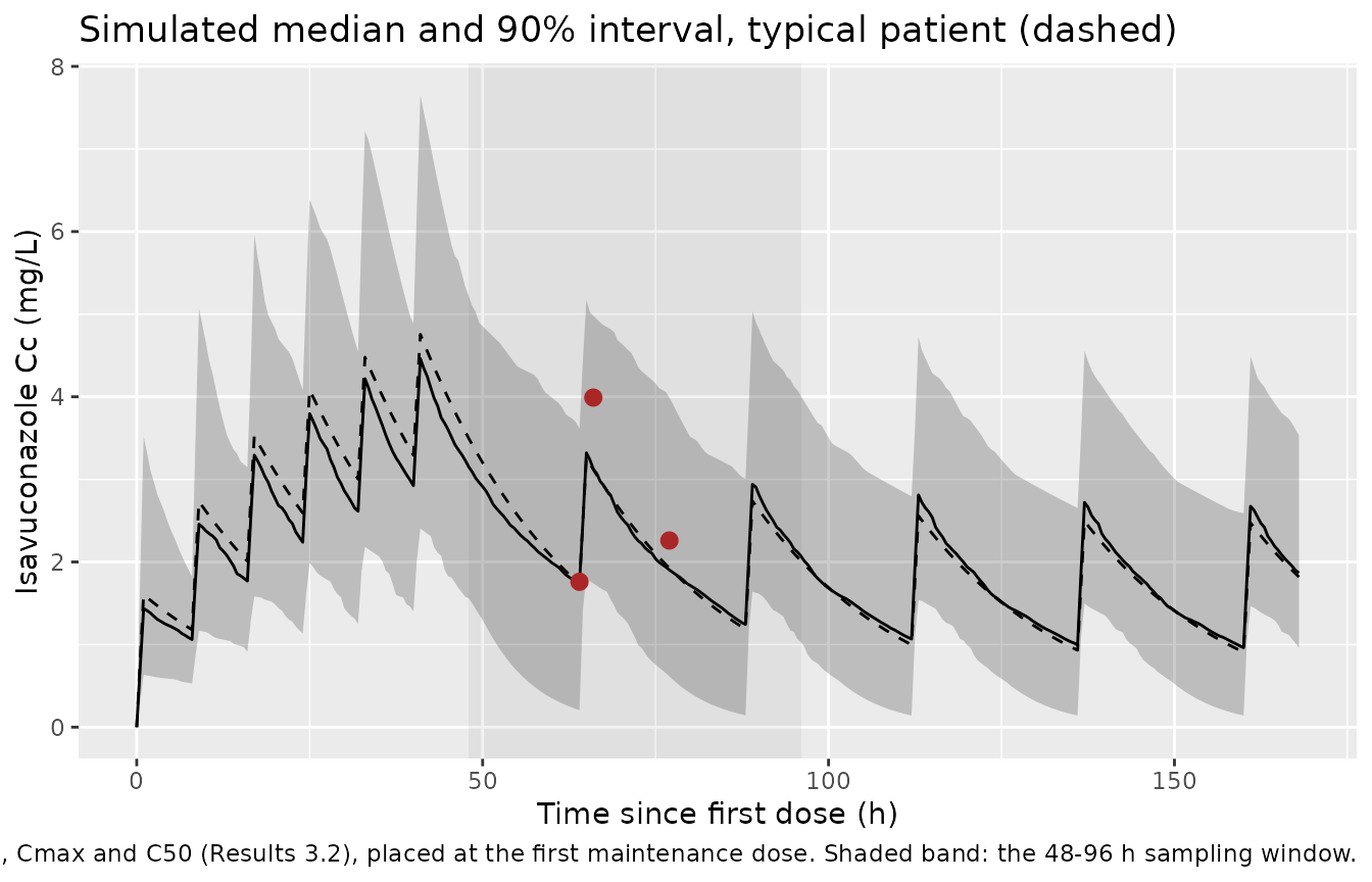
Figure 1 – sampled concentrations
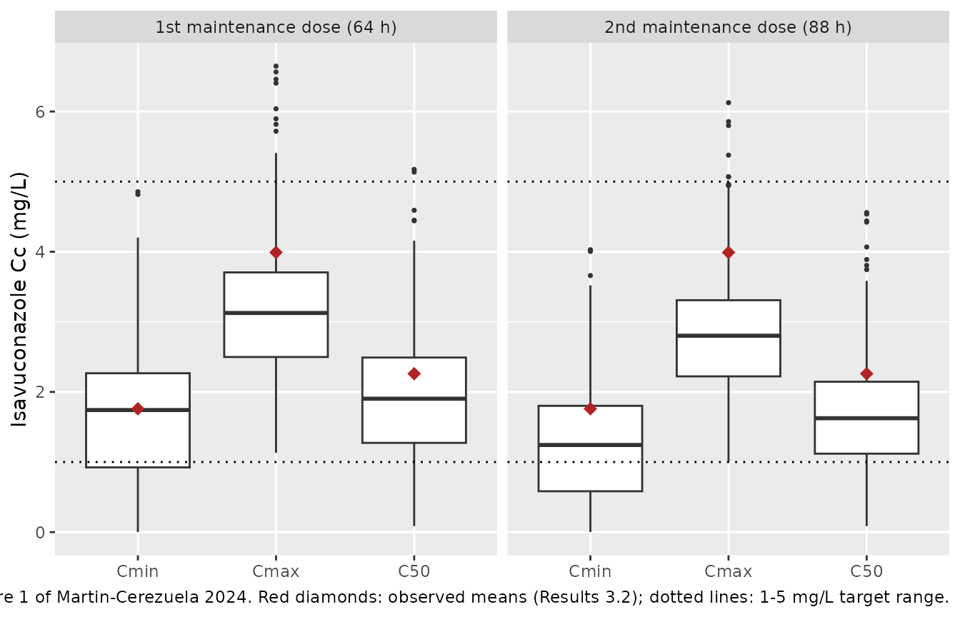
The study sampled each patient once, at predose (Cmin), 1 h (Cmax) and 12 h (C50) after completing an infusion, some time between 48 and 96 h of treatment (Methods 2.2). The regimen puts the first maintenance dose at 64 h and the second at 88 h, so both fall inside that window; the simulation below reads both.
sample_times <- data.frame(
  window = rep(c("1st maintenance dose (64 h)", "2nd maintenance dose (88 h)"), each = 3),
  sample = rep(c("Cmin", "Cmax", "C50"), 2),
  time = c(t_maint + c(0, 2, 13), t_maint + tau + c(0, 2, 13))
)

sampled <- sim |>
  dplyr::inner_join(sample_times, by = "time") |>
  dplyr::mutate(sample = factor(sample, levels = c("Cmin", "Cmax", "C50")))

ggplot(sampled, aes(sample, Cc)) +
  geom_boxplot(outlier.size = 0.6) +
  geom_point(
    data = obs_means |> dplyr::mutate(sample = factor(label, levels = levels(sampled$sample))),
    aes(sample, Cc), colour = "firebrick", size = 3, shape = 18
  ) +
  geom_hline(yintercept = c(1, 5), linetype = 3) +
  facet_wrap(~window) +
  labs(
    x = NULL, y = "Isavuconazole Cc (mg/L)",
    caption = "Replicates Figure 1 of Martin-Cerezuela 2024. Red diamonds: observed means (Results 3.2); dotted lines: 1-5 mg/L target range."
  )
observed <- data.frame(
  sample = c("Cmin", "Cmax", "C50"),
  obs_mean = c(1.76, 3.99, 2.26),
  obs_sd = c(1.02, 1.96, 1.20)
)

sample_cmp <- sampled |>
  dplyr::group_by(window, sample) |>
  dplyr::summarise(
    sim_mean = mean(Cc), sim_sd = sd(Cc),
    pct_below_1 = 100 * mean(Cc < 1),
    .groups = "drop"
  ) |>
  dplyr::mutate(sample = as.character(sample)) |>
  dplyr::left_join(observed, by = "sample") |>
  dplyr::mutate(pct_diff = 100 * (sim_mean / obs_mean - 1))

sample_cmp |>
  dplyr::mutate(
    dplyr::across(c(sim_mean, sim_sd, obs_mean, obs_sd), \(x) round(x, 2)),
    dplyr::across(c(pct_below_1, pct_diff), \(x) round(x, 1))
  ) |>
  dplyr::select(window, sample, obs_mean, obs_sd, sim_mean, sim_sd, pct_diff, pct_below_1) |>
  dplyr::rename(
    "Sampling window" = window,
    "Sample" = sample,
    "Observed mean (mg/L)" = obs_mean,
    "Observed SD" = obs_sd,
    "Simulated mean (mg/L)" = sim_mean,
    "Simulated SD" = sim_sd,
    "% diff (mean)" = pct_diff,
    "Simulated % below 1 mg/L" = pct_below_1
  ) |>
knitr::kable(caption = "Observed (Results 3.2) vs simulated sampled concentrations. 12.5% of observed troughs were below 1 mg/L.")| Sampling window | Sample | Observed mean (mg/L) | Observed SD | Simulated mean (mg/L) | Simulated SD | % diff (mean) | Simulated % below 1 mg/L |
|---|---|---|---|---|---|---|---|
| 1st maintenance dose (64 h) | Cmin | 1.76 | 1.02 | 1.72 | 1.02 | -2.2 | 26.5 |
| 1st maintenance dose (64 h) | Cmax | 3.99 | 1.96 | 3.21 | 1.02 | -19.5 | 0.0 |
| 1st maintenance dose (64 h) | C50 | 2.26 | 1.20 | 1.97 | 0.99 | -12.6 | 15.0 |
| 2nd maintenance dose (88 h) | Cmin | 1.76 | 1.02 | 1.34 | 0.90 | -24.0 | 39.0 |
| 2nd maintenance dose (88 h) | Cmax | 3.99 | 1.96 | 2.86 | 0.92 | -28.3 | 0.5 |
| 2nd maintenance dose (88 h) | C50 | 2.26 | 1.20 | 1.75 | 0.89 | -22.8 | 19.5 |
first_window <- sample_cmp |>
  dplyr::filter(window == "1st maintenance dose (64 h)")
stopifnot(
  # Structural: a mis-transcribed CL, V, dose or infusion time moves every
  # sampled mean by tens of percent. Realised -2 / -20 / -13% for Cmin /
  # Cmax / C50 here; Monte Carlo SE of a 200-subject mean is 2-4%.
  all(abs(first_window$pct_diff) < 35)
)
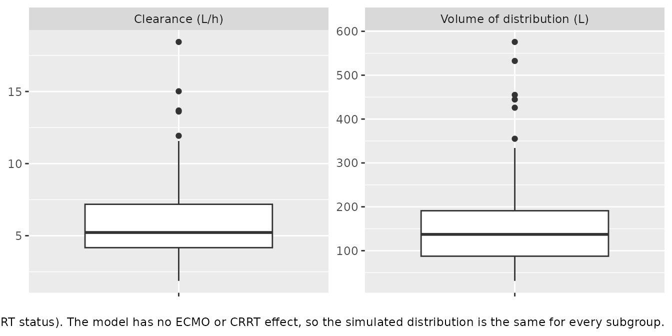
Figure 2 – individual clearance and volume
indiv <- sim |>
  dplyr::distinct(id, cl, vc)

indiv |>
  tidyr::pivot_longer(c(cl, vc), names_to = "parameter", values_to = "value") |>
  dplyr::mutate(parameter = dplyr::recode(
    parameter,
    cl = "Clearance (L/h)", vc = "Volume of distribution (L)"
  )) |>
  ggplot(aes(x = "", y = value)) +
  geom_boxplot() +
  facet_wrap(~parameter, scales = "free_y") +
  labs(
    x = NULL, y = NULL,
    caption = paste(
      "Compare with Figure 2 of Martin-Cerezuela 2024 (individual CL and V by",
      "ECMO and CRRT status). The model has no ECMO or CRRT effect, so the",
      "simulated distribution is the same for every subgroup."
    )
  )
PKNCA validation
Steady-state NCA over the last 24-h dosing interval of the three-week simulation.
sim_nca <- sim |>
  dplyr::filter(!is.na(Cc)) |>
  dplyr::select(id, time, Cc, regimen)

dose_df <- events |>
  dplyr::filter(evid == 1) |>
  dplyr::select(id, time, amt, regimen) |>
  dplyr::mutate(duration = 1)

conc_obj <- PKNCA::PKNCAconc(sim_nca, Cc ~ time | regimen + id)
dose_obj <- PKNCA::PKNCAdose(
  dose_df, amt ~ time | regimen + id,
  route = "intravascular", duration = "duration"
)

intervals <- data.frame(
  start = t_ss,
  end = t_ss + tau,
  cmax = TRUE,
  cmin = TRUE,
  auclast = TRUE,
  cav = TRUE
)

nca_res <- PKNCA::pk.nca(PKNCA::PKNCAdata(conc_obj, dose_obj, intervals = intervals))
summary(nca_res)
#>  start end                         regimen   N     auclast        cmax
#>    544 568 200 mg q8h x6, then 200 mg q24h 200 37.1 [41.4] 2.57 [35.0]
#>         cmin         cav
#>  0.757 [122] 1.55 [41.4]
#>
#> Caption: auclast, cmax, cmin, cav: geometric mean and geometric coefficient of variation; N: number of subjects
Comparison against published NCA
The paper’s only NCA-type quantity is the AUC in Table 2. It is the
typical patient’s dose / CL, which is the population median of the
individual dose / CL values, so it is compared against the median
simulated steady-state AUC0-24 (ncaComparisonTable() pools
by the median).
published <- data.frame(regimen = "200 mg q8h x6, then 200 mg q24h", auclast = 37.31)

cmp <- nlmixr2lib::ncaComparisonTable(
  simulated = nca_res,
  reference = published,
  by = "regimen",
  params = "auclast",
  units = c(auclast = "mg*h/L"),
  tolerance_pct = 20
)
knitr::kable(cmp, caption = "Steady-state AUC0-24: published (Table 2) vs simulated median.")| NCA parameter | regimen | Reference | Simulated | % diff |
|---|---|---|---|---|
| AUClast (mg*h/L) | 200 mg q8h x6, then 200 mg q24h | 37.3 | 38.3 | +2.7% |
auc_ss <- as.data.frame(nca_res) |>
  dplyr::filter(PPTESTCD == "auclast")
stopifnot(
  # Median of dose / CL_i is dose / CL_typ for a lognormal CL; Monte Carlo
  # SE of the median from 200 subjects is about 4%.
  abs(median(auc_ss$PPORRES) / 37.31 - 1) < 0.15
)
Assumptions and deviations
-
Residual error. Neither the article nor its
Research Square preprint reports a residual error model or its
magnitude. Proportional and additive residual SDs are carried as
fixed(0)rather than invented, so simulations from this model show between-subject variability only. -
IIV scale. Table 2’s
%CVcolumn (the preprint footnote calls it “percent covariance of intersubject-variability”) is converted with omega^2 = log(CV^2 + 1), giving 0.1867 for CL and 0.3708 for V. The paper does not say whether its %CV is instead 100 x sqrt(omega^2), which would give 0.2052 and 0.4489. No confidence interval on the variances is printed, so the two readings cannot be separated from the paper; the difference in the SD of log(CL) is under 5% and in log(V) about 10%. - Table 2 RSE for clearance. The printed %RSE of 35.7% for clearance does not match its own SE (0.576 / 5.36 = 10.7%) or its 95% CI (5.36 +/- 1.96 x 0.576 = 4.23-6.49). The point estimate, SE and CI agree, so the point estimate is used as printed.
- Start of maintenance dosing. Methods 2.1 gives six 200 mg loading doses every 8 h followed by 200 mg every 24 h without saying when the first maintenance dose falls. The simulation starts it 24 h after the last loading dose (at 64 h), the later end of the 12-24 h interval in the product label.
- Sampling times. Methods 2.2 places Cmax and C50 at 1 h and 12 h “after completing the drug infusion” (simulated at 2 h and 13 h after the start of the 1-h infusion); the abstract says “after the last dose”. The study does not say on which day within 48-96 h each patient was sampled, so the first two maintenance doses are both shown. Observed means sit closest to the first-maintenance-dose window (simulated Cmin within a few percent, Cmax about 20% lower); at the second window all three simulated means are about 23-28% lower, consistent with most patients having been sampled soon after the loading phase.
- Spread of the simulated concentrations. With no residual error, the simulated concentrations carry between-subject variability only. The simulated SD of Cmax (about 1 mg/L) is about half the observed SD (1.96 mg/L), and the simulated fraction of troughs below 1 mg/L (about a quarter at the first window) is higher than the observed 12.5% (3 of 24), which a 24-patient sample estimates only coarsely.
-
Covariate units in Table 1. Table 1 prints
bilirubin in umol/L (mean 1.1) and albumin in g/L (mean 2.4); both
magnitudes are mg/dL and g/dL values. They are documented that way in
covariatesDataExcluded; no covariate enters the model. - ECMO and CRRT. The authors tested both on CL and V and retained neither (Results 3.3, Figure 2), so the model applies to patients on and off these devices alike.