Levetiracetam in term and preterm neonates (Johnson 2025)
Source:vignettes/articles/Johnson_2025_levetiracetam.Rmd
Johnson_2025_levetiracetam.RmdModel and source
- Citation: Johnson A, Thomas N, Blumenthal M, Ikonomidou C, Lim SY. A Physiologically Based Modeling Approach to Evaluate Intravenous Levetiracetam Dosing in Term and Preterm Neonates. J Clin Pharmacol. 2025;65(10):1246. doi:10.1002/jcph.70037
- Description: One-compartment reduction of the Johnson 2025 neonatal physiologically based pharmacokinetic (PBPK) model of intravenous levetiracetam in term and preterm neonates (Simcyp V23 full PBPK). Volume is the paper’s neonatal steady-state volume (0.96 L/kg, Kp scalar 1.56). Total clearance is the sum of the paper’s two neonatal clearance equations: renal clearance scaled from the adult value by the Wu 2022 neonatal GFR model (birth weight, gestational age and postnatal age) times a maturation factor of 1.61, and metabolic (Type B esterase) clearance scaled allometrically (exponent 0.75) from the adult value times a quadratic ontogeny function of postmenstrual age, floored at zero. Typical-value model: no between-subject or residual variability.
- Article: https://doi.org/10.1002/jcph.70037 (open access, https://www.ncbi.nlm.nih.gov/pmc/articles/PMC12484410/)
What this model is, and what it is not
Johnson 2025 built a whole-body PBPK model of levetiracetam in Simcyp V23, stepping from adults to children to term and preterm neonates. The whole-body distribution equations and the virtual-population physiology are part of the Simcyp platform and are not printed, so the platform model itself cannot be encoded.
What the paper does print is everything that sets the neonatal exposure of this drug:
- the neonatal steady-state volume, 0.96 L/kg (Table 1, after a Kp scalar of 1.56);
- the neonatal renal clearance equation: adult renal clearance (2.64 L/h) scaled by the Wu 2022 neonatal GFR model and a maturation factor of 1.61 (Table 1 footnote e, Methods);
- the neonatal metabolic clearance equation: adult metabolic clearance (1.36 L/h) scaled allometrically with exponent 0.75 and an empirical quadratic ontogeny function of postmenstrual age (Table 1 footnote c, Figure 2a).
Levetiracetam is hydrophilic (logP -0.64), almost unbound (fu 0.966), and is described by a one-compartment model in every neonatal popPK study the paper cites (Table 2). This package therefore ships a one-compartment reduction with the paper’s volume and its two clearance equations. The sections below show that it reproduces the paper’s own predicted clearances (Table S6) to within 9% and its predicted 96-h troughs (Table S7) to within the gap expected between a typical value and a virtual-population mean.
Two things the reduction does not do:
- It does not reproduce the PBPK distribution phase. The peaks drawn in Figures 4-6 sit above a one-compartment peak, because the PBPK model fills the well-perfused organs first. Troughs, average concentrations and clearance are unaffected.
- It is a typical-value model. The 5th-95th percentile bands in the paper’s figures come from Simcyp virtual-population physiology (organ sizes, GFR, tissue-volume CVs of 20-45%), which is not reported.
Population
There is no fitted population: this is a PBPK model. The neonatal layer was calibrated against Sharpe 2012 (18 term neonates, GA 36-41 weeks, PNA 1-5 days, 2.5-4.7 kg) and evaluated against Sharpe 2024 (49 term neonates), Merhar 2011 (18 neonates, GA 35-41 weeks, PNA 0-32 days) and Lima-Rogel 2018 (20 neonates, GA 28-40.3 weeks, PNA 3-25 days, 0.9-3.75 kg) (Johnson 2025 Table 2). Simulations used Simcyp Sim-Pediatric (term) and Sim-Preterm virtual populations of 500 subjects.
Source trace
| Quantity | Value | Source |
|---|---|---|
Neonatal Vss (lvc) |
0.96 L/kg | Table 1, Neonatal Model column; footnote b (Kp scalar 1.56) |
Adult renal clearance (lcl_renal) |
2.64 L/h | Table 1; Methods “Adult PBPK Model Development” |
Adult metabolic clearance (lcl_nonren) |
1.36 L/h | Table 1; Equation 1 |
Renal maturation factor (mf_renal) |
1.61 | Table 1 footnote e (Equation 2); Results; Figure 2b |
Adult GFR reference (lgfr_adult) |
6.9 L/h | Not printed; back-solved from Table S6 (below) |
Wu 2022 GFR: scale (lgfr_bw) |
0.086 L/h | Methods GFR equation |
Wu 2022 GFR: postnatal coefficient (gfr_pna_frac) |
0.154 | Methods GFR equation |
Wu 2022 GFR: GA exponent (e_ga_gfr) |
9.99 | Methods GFR equation |
Wu 2022 GFR: GA exponent on the PNA power
(e_ga_gfr_pnaexp) |
-1.71 | Methods GFR equation |
Allometric exponent (e_wt_cl_nonren) |
0.75 | Table 1; Equation 1; Methods |
Ontogeny function (of_pma2, of_pma1,
of_int) |
-0.0716, 5.808, -117.1 | Figure 2a (see erratum below) |
| Renal clearance equation | CL_R = 2.64 x GFR_neonate / GFR_adult x 1.61 | Table 1 footnote e; Methods |
| Metabolic clearance equation | CL_M = 1.36 x (WT/70)^0.75 x OF | Table 1 footnote c; Methods |
| GFR equation | 0.086 x [bW/1.75 + (GA/34)^9.99 x 0.154 x (PNA/2)((GA/34)-1.71)] | Methods, “PBPK Model Scaling to Term Neonates” |
| Floor of OF at zero | – | Results: metabolic clearance “low to nonexistent at PMA of <37.5 weeks” |
Erratum: the ontogeny function
Table 1 footnote c and the Results equation print the ontogeny
function as OF = -0.716 x PMA^2 + 5.808 x PMA - 177.1. That
gives an ontogeny factor below -900 at term, which cannot be what was
simulated. Figure 2a prints it as
OF = -0.0716 x PMA^2 + 5.808 x PMA - 117.1, and that form
matches every statement in the text: about 20% of the allometric
clearance at 38 weeks, about 60% at 40 weeks, and zero below about 37.5
weeks. The model uses the Figure 2a form.
of_fig <- function(pma) -0.0716 * pma^2 + 5.808 * pma - 117.1
of_tab <- function(pma) -0.716 * pma^2 + 5.808 * pma - 177.1
knitr::kable(
  data.frame(pma = c(37.5, 38, 39, 40)) |>
    dplyr::mutate(fig = round(of_fig(pma), 3), tab = round(of_tab(pma), 1)) |>
    dplyr::rename(
      "PMA (weeks)" = pma,
      "OF, Figure 2a form" = fig,
      "OF, Table 1 / text form" = tab
    ),
  caption = "Ontogeny function at the PMAs the Results text describes."
)| PMA (weeks) | OF, Figure 2a form | OF, Table 1 / text form |
|---|---|---|
| 37.5 | 0.012 | -966.2 |
| 38.0 | 0.214 | -990.3 |
| 39.0 | 0.508 | -1039.6 |
| 40.0 | 0.660 | -1090.4 |
ggplot(data.frame(pma = seq(36, 45, by = 0.05)),
       aes(pma, pmax(of_fig(pma), 0))) +
  geom_line(colour = "darkgreen", linewidth = 1) +
  annotate("rect", xmin = 38, xmax = 40, ymin = -Inf, ymax = Inf, alpha = 0.1) +
  labs(x = "Postmenstrual age (weeks)",
       y = "Ontogeny factor OF (floored at 0)",
       caption = "Shaded: PMA range of Figure 2a (Sharpe 2012 term neonates)") +
  theme_bw()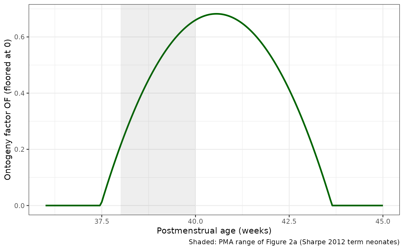
Replicates the green line of Figure 2a of Johnson 2025 (fraction of the allometrically scaled metabolic clearance retained), extended to the whole neonatal PMA range. The quadratic peaks at 40.6 weeks and returns to zero at about 43.6 weeks; the model floors it at zero.
The adult GFR reference
Equation 2 divides by GFR_adult, Simcyp’s adult
reference GFR, whose value the paper does not print. Every other input
is printed, so the one missing value can be read off the paper’s own
output: Table S6 lists the predicted weight-normalised clearance at the
end of the first and second weeks of life for GA 28, 31, 35 and 38
weeks. With approximate median birth weights for each GA, the single
value of GFR_adult that best reproduces those eight numbers
is 6.9 L/h (115 mL/min). It moves only between 6.8 and 7.1 L/h when
every birth weight is shifted by 0.15 kg either way. One value fitting
all eight cells across a four-fold range of clearance shows that the
printed GFR equation, the maturation factor and the corrected ontogeny
function are mutually consistent.
Virtual cohort
The paper’s virtual neonates come from Simcyp population files whose birth-weight-by-GA table is not printed. This vignette uses one typical neonate per gestational age, with a birth weight close to the median for that GA, and holds body weight at birth weight. (Simcyp grows the simulated neonates over the simulated week; a few percent of weight gain changes neither clearance nor troughs materially.)
mod <- readModelDb("Johnson_2025_levetiracetam")

typical <- tibble::tribble(
  ~GA, ~WT_BIRTH,
   28,  1.10,
   31,  1.60,
   35,  2.45,
   38,  3.15
)
days_per_month <- 30.4375

# One record per time point; PNA (months) is time-varying.
make_obs <- function(ga, bw, pna0_d, times, id) {
  data.frame(
    id = id, time = times, evid = 0L, amt = 0, rate = 0, cmt = "central",
    GA = ga, WT_BIRTH = bw, WT = bw,
    PNA = (pna0_d + times / 24) / days_per_month
  )
}
Clearance against Table S6
The model’s cl output is the instantaneous total
clearance. Evaluating it at postnatal day 7 and day 14 reproduces Table
S6.
s6 <- tibble::tribble(
  ~GA, ~pna_d, ~paper_ml_min_kg,
   38,     7,  1.28,
   35,     7,  0.74,
   31,     7,  0.64,
   28,     7,  0.58,
   38,    14,  1.50,
   35,    14,  1.00,
   31,    14,  0.86,
   28,    14,  0.79
) |>
  dplyr::left_join(typical, by = "GA") |>
  dplyr::mutate(id = dplyr::row_number())

ev_s6 <- do.call(rbind, lapply(seq_len(nrow(s6)), function(i) {
  make_obs(s6$GA[i], s6$WT_BIRTH[i], s6$pna_d[i], 0, s6$id[i])
}))
cl_s6 <- as.data.frame(rxode2::rxSolve(mod, ev_s6, returnType = "data.frame"))
#> Warning: multi-subject simulation without without 'omega'

s6_cmp <- s6 |>
  dplyr::left_join(cl_s6 |> dplyr::select(id, cl, cl_renal, cl_nonren), by = "id") |>
  dplyr::mutate(
    model_ml_min_kg = cl / WT_BIRTH * 1000 / 60,
    pct_diff = 100 * (model_ml_min_kg / paper_ml_min_kg - 1)
  )

knitr::kable(
  s6_cmp |>
    dplyr::transmute(
      GA, pna_d, WT_BIRTH,
      renal = round(cl_renal, 3), metabolic = round(cl_nonren, 3),
      model = round(model_ml_min_kg, 2), paper = paper_ml_min_kg,
      pct = round(pct_diff, 1)
    ) |>
    dplyr::rename(
      "GA (weeks)" = GA, "PNA (days)" = pna_d, "Weight (kg)" = WT_BIRTH,
      "CL renal (L/h)" = renal, "CL metabolic (L/h)" = metabolic,
      "Model CL (mL/min/kg)" = model, "Table S6 (mL/min/kg)" = paper,
      "% diff" = pct
    ),
  caption = "Weight-normalised total clearance: model vs Johnson 2025 Table S6."
)| GA (weeks) | PNA (days) | Weight (kg) | CL renal (L/h) | CL metabolic (L/h) | Model CL (mL/min/kg) | Table S6 (mL/min/kg) | % diff |
|---|---|---|---|---|---|---|---|
| 38 | 7 | 3.15 | 0.165 | 0.068 | 1.23 | 1.28 | -3.8 |
| 35 | 7 | 2.45 | 0.110 | 0.000 | 0.75 | 0.74 | 1.2 |
| 31 | 7 | 1.60 | 0.062 | 0.000 | 0.65 | 0.64 | 1.7 |
| 28 | 7 | 1.10 | 0.040 | 0.000 | 0.61 | 0.58 | 4.6 |
| 38 | 14 | 3.15 | 0.219 | 0.088 | 1.62 | 1.50 | 8.3 |
| 35 | 14 | 2.45 | 0.144 | 0.000 | 0.98 | 1.00 | -2.3 |
| 31 | 14 | 1.60 | 0.080 | 0.000 | 0.83 | 0.86 | -3.0 |
| 28 | 14 | 1.10 | 0.051 | 0.000 | 0.77 | 0.79 | -2.3 |
# Deterministic typical-value evaluation, so a bound on every cell is safe.
stopifnot(all(abs(s6_cmp$pct_diff) < 10), abs(median(s6_cmp$pct_diff)) < 5)
Metabolic clearance is zero below 37.5 weeks PMA, so in the three preterm groups the model clearance is renal clearance alone – the paper’s headline finding that preterm neonates clear levetiracetam by the kidney only.
Simulation of the dosing regimens (Figure 5)
Three regimens, each over 7 days, all as 15-min infusions (Johnson 2025 Methods, “Dose-Exposure Assessment”):
- 60 mg/kg loading dose, then 25 mg/kg every 12 h;
- 60 + 60 mg/kg loading doses (the second starting 15 min after the first ends), then 25 mg/kg every 12 h;
- 60 + 60 + 30 mg/kg loading doses, then 25 mg/kg every 8 h.
The first maintenance dose is given one dosing interval after the start of the first loading dose. Simulations start at postnatal day 3, the middle of the paper’s day 1-5 range.
regimens <- list(
  "Regimen 1: 60 LD + 25 q12h" = list(ld_t = 0, ld_amt = 60, tau = 12),
  "Regimen 2: 120 LD + 25 q12h" = list(ld_t = c(0, 0.5), ld_amt = c(60, 60), tau = 12),
  "Regimen 3: 150 LD + 25 q8h" = list(ld_t = c(0, 0.5, 1), ld_amt = c(60, 60, 30), tau = 8)
)

make_doses <- function(ga, bw, pna0_d, reg, id, md = 25, tend = 168) {
  md_t <- seq(reg$tau, tend - 1e-6, by = reg$tau)
  t <- c(reg$ld_t, md_t)
  amt <- c(reg$ld_amt, rep(md, length(md_t))) * bw
  data.frame(
    id = id, time = t, evid = 1L, amt = amt, rate = amt / 0.25, cmt = "central",
    GA = ga, WT_BIRTH = bw, WT = bw,
    PNA = (pna0_d + t / 24) / days_per_month
  )
}

grid <- tidyr::expand_grid(typical, regimen = names(regimens)) |>
  dplyr::mutate(id = dplyr::row_number())
obs_times <- sort(unique(c(seq(0, 168, by = 0.25), 96)))

ev_reg <- do.call(rbind, lapply(seq_len(nrow(grid)), function(i) {
  g <- grid[i, ]
  rbind(
    make_doses(g$GA, g$WT_BIRTH, 3, regimens[[g$regimen]], g$id),
    make_obs(g$GA, g$WT_BIRTH, 3, obs_times, g$id)
  )
})) |>
  dplyr::arrange(id, time, dplyr::desc(evid))

sim_reg <- as.data.frame(rxode2::rxSolve(mod, ev_reg, returnType = "data.frame")) |>
  dplyr::left_join(grid |> dplyr::select(id, regimen), by = "id")
#> Warning: multi-subject simulation without without 'omega'
ggplot(sim_reg, aes(time / 24, Cc, colour = regimen)) +
  geom_line() +
  geom_hline(yintercept = 80, linetype = "dashed") +
  geom_hline(yintercept = 50, linetype = "dotted") +
  facet_wrap(~ paste("GA", GA, "weeks")) +
  labs(x = "Time (days)", y = "Levetiracetam (mg/L)", colour = NULL) +
  theme_bw() +
  theme(legend.position = "bottom")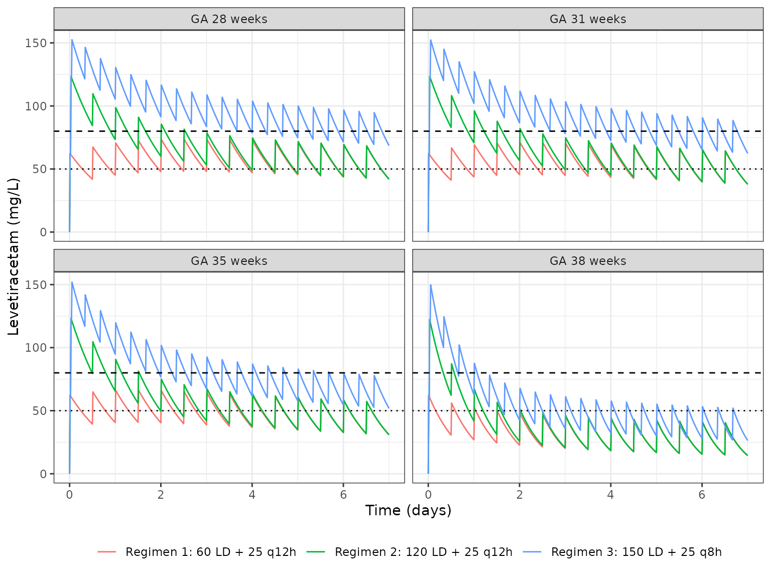
Replicates the mean lines of Figure 5 of Johnson 2025 (typical neonate per GA). Dashed: 80 mg/L random-concentration toxicity reference; dotted: 50 mg/L trough toxicity reference. The PBPK model’s early distribution phase makes the published peaks higher than these one-compartment peaks; troughs are directly comparable.
Trough concentrations at 96 h (Table S7)
Table S7 reports the mean 96-h trough over 500 virtual neonates per GA for Regimen 1, plus three reduced maintenance doses the paper proposes for preterm neonates.
s7_extra <- tibble::tribble(
  ~GA, ~md,
   35, 12.5,
   31, 10,
   28,  8
) |>
  dplyr::left_join(typical, by = "GA") |>
  dplyr::mutate(id = 100L + dplyr::row_number())

ev_s7 <- do.call(rbind, lapply(seq_len(nrow(s7_extra)), function(i) {
  g <- s7_extra[i, ]
  rbind(
    make_doses(g$GA, g$WT_BIRTH, 3, regimens[[1]], g$id, md = g$md),
    make_obs(g$GA, g$WT_BIRTH, 3, 96, g$id)
  )
})) |>
  dplyr::arrange(id, time, dplyr::desc(evid))
sim_s7 <- as.data.frame(rxode2::rxSolve(mod, ev_s7, returnType = "data.frame"))
#> Warning: multi-subject simulation without without 'omega'

# A dose is given at 96 h in every regimen 1 arm; the observation sorted
# after the dose record is still the pre-infusion trough because the
# infusion has not yet delivered any drug at t = 96.
trough <- dplyr::bind_rows(
  sim_reg |>
    dplyr::filter(regimen == names(regimens)[1], time == 96) |>
    dplyr::transmute(GA, md = 25, model = Cc),
  sim_s7 |>
    dplyr::filter(time == 96) |>
    dplyr::left_join(s7_extra |> dplyr::select(id, md), by = "id") |>
    dplyr::transmute(GA, md, model = Cc)
) |>
  dplyr::distinct(GA, md, .keep_all = TRUE)

s7 <- tibble::tribble(
  ~GA, ~md,  ~paper_mean, ~paper_sd,
   38, 25,   19.24,        6.32,
   35, 25,   42.52,       17.87,
   31, 25,   50.30,       19.64,
   28, 25,   55.87,       21.10,
   35, 12.5, 24.97,       11.07,
   31, 10,   21.85,        9.55,
   28,  8,   20.16,        8.89
) |>
  dplyr::left_join(trough, by = c("GA", "md")) |>
  dplyr::mutate(ratio = model / paper_mean)

knitr::kable(
  s7 |>
    dplyr::mutate(model = round(model, 1), ratio = round(ratio, 2)) |>
    dplyr::rename(
      "GA (weeks)" = GA, "Maintenance dose (mg/kg q12h)" = md,
      "Table S7 mean (mg/L)" = paper_mean, "Table S7 SD (mg/L)" = paper_sd,
      "Typical-neonate trough (mg/L)" = model, "Model / paper mean" = ratio
    ),
  caption = "96-h trough after a 60 mg/kg loading dose: typical neonate vs Johnson 2025 Table S7 virtual-population mean."
)| GA (weeks) | Maintenance dose (mg/kg q12h) | Table S7 mean (mg/L) | Table S7 SD (mg/L) | Typical-neonate trough (mg/L) | Model / paper mean |
|---|---|---|---|---|---|
| 38 | 25.0 | 19.24 | 6.32 | 18.3 | 0.95 |
| 35 | 25.0 | 42.52 | 17.87 | 36.7 | 0.86 |
| 31 | 25.0 | 50.30 | 19.64 | 43.4 | 0.86 |
| 28 | 25.0 | 55.87 | 21.10 | 47.0 | 0.84 |
| 35 | 12.5 | 24.97 | 11.07 | 19.2 | 0.77 |
| 31 | 10.0 | 21.85 | 9.55 | 18.6 | 0.85 |
| 28 | 8.0 | 20.16 | 8.89 | 16.6 | 0.82 |
stopifnot(
  # Centre: the typical value sits a little below the mean of a skewed
  # (CV 33-46%) virtual-population trough distribution.
  median(s7$ratio) > 0.75, median(s7$ratio) < 1.05,
  # Envelope: deterministic, so every cell can be bounded.
  all(s7$ratio > 0.65), all(s7$ratio < 1.1)
)
The typical-neonate trough is 0.77-0.95 of the published mean. A shortfall of this size is expected: trough concentration varies roughly as 1/CL, so with the 33-46% CV of Table S7 the population mean lies 10-20% above the trough of a subject with typical clearance. The ordering by GA, and the size of the maintenance-dose reduction needed to bring preterm troughs back to the term level, are reproduced.
First versus second week of life (Figure 6)
ev_wk <- do.call(rbind, lapply(seq_len(nrow(typical)), function(i) {
  g <- typical[i, ]
  do.call(rbind, lapply(c(3, 10), function(p0) {
    id <- 200L + 10L * i + p0
    rbind(
      make_doses(g$GA, g$WT_BIRTH, p0, regimens[[1]], id),
      make_obs(g$GA, g$WT_BIRTH, p0, seq(0, 168, by = 0.25), id)
    )
  }))
})) |>
  dplyr::arrange(id, time, dplyr::desc(evid))

sim_wk <- as.data.frame(rxode2::rxSolve(mod, ev_wk, returnType = "data.frame")) |>
  dplyr::mutate(week = ifelse(id %% 10L == 3L, "First week (start PNA 3 d)",
                              "Second week (start PNA 10 d)"))
#> Warning: multi-subject simulation without without 'omega'

ggplot(sim_wk, aes(time / 24, Cc, colour = week)) +
  geom_line() +
  geom_hline(yintercept = 80, linetype = "dashed") +
  geom_hline(yintercept = 50, linetype = "dotted") +
  facet_wrap(~ paste("GA", GA, "weeks")) +
  labs(x = "Time (days)", y = "Levetiracetam (mg/L)", colour = NULL) +
  theme_bw() +
  theme(legend.position = "bottom")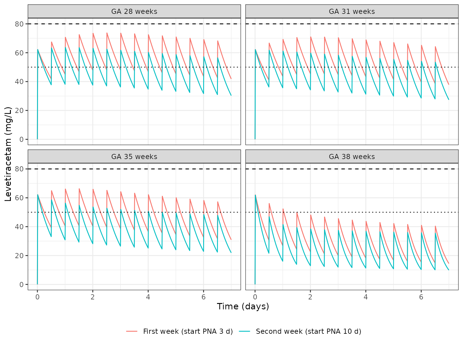
Replicates the mean lines of Figure 6 of Johnson 2025: Regimen 1 started on postnatal day 3 (first week) or day 10 (second week), typical neonate per GA.
PKNCA validation
Table S3 reports the paper’s predicted clearance and volume at the Sharpe 2012 setting (term neonates, GA 37-40 weeks, clearance evaluated at postnatal day 7). The NCA below gives a single 20 mg/kg 15-min infusion to a typical GA 39-week, 3.4-kg neonate held at postnatal day 7, so clearance is constant over the profile.
bw_term <- 3.4
ev_nca <- rbind(
  data.frame(
    id = 1L, time = 0, evid = 1L, amt = 20 * bw_term, rate = 20 * bw_term / 0.25,
    cmt = "central", GA = 39, WT_BIRTH = bw_term, WT = bw_term,
    PNA = 7 / days_per_month
  ),
  data.frame(
    id = 1L, time = c(0, 0.25, 0.5, 1, 2, 4, 8, 12, 24, 36, 48, 72, 96, 120),
    evid = 0L, amt = 0, rate = 0, cmt = "central", GA = 39,
    WT_BIRTH = bw_term, WT = bw_term, PNA = 7 / days_per_month
  )
) |>
  dplyr::mutate(treatment = "20 mg/kg, GA 39 weeks, PNA 7 days")

# A single-subject solve returns no `id` column; add it back with the arm label.
sim_nca <- as.data.frame(rxode2::rxSolve(mod, ev_nca, returnType = "data.frame")) |>
  dplyr::mutate(id = 1L, treatment = unique(ev_nca$treatment))

conc_nca <- sim_nca |>
  dplyr::filter(!is.na(Cc)) |>
  dplyr::select(id, time, Cc, treatment)
conc_nca <- dplyr::bind_rows(
  conc_nca,
  conc_nca |> dplyr::distinct(id, treatment) |> dplyr::mutate(time = 0, Cc = 0)
) |>
  dplyr::distinct(id, treatment, time, .keep_all = TRUE) |>
  dplyr::arrange(id, treatment, time)

dose_nca <- ev_nca |>
  dplyr::filter(evid == 1L) |>
  dplyr::mutate(duration = 0.25) |>
  dplyr::select(id, time, amt, duration, treatment)

nca_obj <- PKNCA::pk.nca(PKNCA::PKNCAdata(
  PKNCA::PKNCAconc(conc_nca, Cc ~ time | treatment + id, concu = "mg/L", timeu = "h"),
  PKNCA::PKNCAdose(dose_nca, amt ~ time | treatment + id, doseu = "mg",
                   duration = "duration", route = "intravascular"),
  intervals = data.frame(start = 0, end = Inf, cmax = TRUE, aucinf.obs = TRUE,
                         half.life = TRUE, cl.obs = TRUE, vss.obs = TRUE)
))

nca_res <- as.data.frame(nca_obj) |>
  dplyr::filter(PPTESTCD %in% c("cmax", "aucinf.obs", "half.life", "cl.obs", "vss.obs"))
knitr::kable(nca_res |> dplyr::mutate(PPORRES = signif(PPORRES, 4)) |>
               dplyr::select(treatment, PPTESTCD, PPORRES),
caption = "PKNCA results (absolute units).")| treatment | PPTESTCD | PPORRES |
|---|---|---|
| 20 mg/kg, GA 39 weeks, PNA 7 days | cmax | 20.6100 |
| 20 mg/kg, GA 39 weeks, PNA 7 days | half.life | 8.0140 |
| 20 mg/kg, GA 39 weeks, PNA 7 days | aucinf.obs | 240.9000 |
| 20 mg/kg, GA 39 weeks, PNA 7 days | cl.obs | 0.2823 |
| 20 mg/kg, GA 39 weeks, PNA 7 days | vss.obs | 3.3000 |
# Weight-normalise clearance (mL/min/kg) and volume (L/kg) to match Table S3.
sim_kg <- nca_res |>
  dplyr::filter(PPTESTCD %in% c("cl.obs", "vss.obs")) |>
  dplyr::mutate(
    PPORRES = ifelse(PPTESTCD == "cl.obs", PPORRES / bw_term * 1000 / 60,
                     PPORRES / bw_term)
  )

cmp <- nlmixr2lib::ncaComparisonTable(
  simulated = sim_kg,
  reference = tibble::tibble(treatment = unique(sim_kg$treatment),
                             cl.obs = 1.37, vss.obs = 0.95),
  by = "treatment",
  units = c(cl.obs = "mL/min/kg", vss.obs = "L/kg"),
  tolerance_pct = 20
)
knitr::kable(cmp, caption = paste(
  "Model vs Johnson 2025 Table S3 predicted mean for the Sharpe 2012 setting",
  "(clearance at PNA day 7). * differs from the reference by >20%."
))| NCA parameter | treatment | Reference | Simulated | % diff |
|---|---|---|---|---|
| CL/F (mL/min/kg) | 20 mg/kg, GA 39 weeks, PNA 7 days | 1.37 | 1.38 | +1.0% |
| Vss/F (L/kg) | 20 mg/kg, GA 39 weeks, PNA 7 days | 0.95 | 0.971 | +2.2% |
pct <- suppressWarnings(as.numeric(gsub("[^0-9.eE+-]", "", as.character(cmp[["% diff"]]))))
stopifnot(sum(is.finite(pct)) == 2, max(abs(pct), na.rm = TRUE) < 15)
Clearance and volume agree with the paper’s predicted Sharpe 2012 values. The paper’s predicted mean is over neonates with GA 37-40 weeks and a range of birth weights, so a single typical neonate is not expected to match it exactly.
Assumptions and deviations
- Model class. The Simcyp whole-body PBPK model is reduced to one compartment with the paper’s neonatal Vss and its two printed clearance equations. The early distribution phase of the PBPK model, which raises the peak after each infusion, is not reproduced; troughs, average concentrations and clearance are.
-
Adult GFR reference.
GFR_adultin Equation 2 is a Simcyp population value that the paper does not print. The model uses 6.9 L/h (115 mL/min), the value that best reproduces the paper’s Table S6 clearances given the other printed inputs. -
Ontogeny function. The Figure 2a form
(
-0.0716,-117.1) is used in place of the Table 1 footnote c / Results form (-0.716,-177.1), which gives impossible values (see Erratum above). - Floor at zero. The quadratic ontogeny function is negative below about 37.5 weeks and above about 43.6 weeks PMA. The model floors it at zero, following the paper’s statement that metabolic clearance is “low to nonexistent” below 37.5 weeks. The paper does not discuss PMA above 41 weeks; above about 43.6 weeks the floored function removes metabolic clearance again, which is an artefact of extrapolating the quadratic beyond its calibration range (PMA 38-40 weeks). Use the model with care for term neonates older than about three weeks.
- GFR equation. The Wu 2022 neonatal GFR model is used exactly as printed in Johnson 2025 (in L/h; birth weight in kg, GA in weeks, PNA in days). The source article (Wu Y et al., AAPS J 2022;24:38) was not consulted; agreement with Table S6 across GA 28-38 weeks supports the printed form.
- Covariates. The paper used Simcyp’s average birth weight for each GA and grew the virtual neonates over the simulation. This vignette uses approximate median birth weights (1.10, 1.60, 2.45 and 3.15 kg at GA 28, 31, 35 and 38 weeks) and holds weight at birth weight.
- Regimen timing. The first maintenance dose is given one dosing interval after the start of the first loading dose; the paper does not say when the maintenance doses start.
- Variability. No between-subject or residual variability is reported for a PBPK model; the residual error is fixed at zero.
-
Not reproduced. The adult and paediatric models
(Tables S1-S2) depend on Simcyp’s paediatric GFR model and on PBPK
absorption, neither of which is printed; Table S5 (reduced GFR) is
reproducible by raising
lgfr_adult(renal clearance scales withGFR_neonate / GFR_adult), and the Table S4 comparison against Lima-Rogel 2018 requires that study’s GA-specific covariates, which are not printed.