Tilmicosin PK/PD against Pasteurella multocida (Chen 2023)
Source:vignettes/articles/Chen_2023_tilmicosin.Rmd
Chen_2023_tilmicosin.RmdModel and source
- Citation: Chen Y, Ji X, Zhang S, Wang W, Zhang H, Ding H. (2023). Pharmacokinetic/pharmacodynamic integration of tilmicosin against Pasteurella multocida in a piglet tissue cage model. Frontiers in Veterinary Science 10:1260990.
- Article: https://doi.org/10.3389/fvets.2023.1260990
This vignette validates the packaged model
Chen_2023_tilmicosin against the published Chen 2023
results.
Chen 2023 implanted silicone tissue cages subcutaneously in piglets, infected them with P. multocida serovar D:7, dosed tilmicosin orally at 30, 40, 50 or 60 mg/kg once daily for three days, and related the drug exposure inside the cage to the change in bacterial count. The PK/PD integration is a sigmoidal Emax model on a PK/PD index (Section 2.6):
where E is the change in bacterial count (log10 CFU/mL)
over a 24 h dosing interval, E0 is the corresponding change
in the untreated control, and Ce is a PK/PD index. Chen
2023 evaluated three candidate indices and found AUC24h/MIC
to correlate best with effect (R^2 = 0.92, versus 0.90 for
Cmax/MIC and 0.83 for %T>MIC); Table 2
reports parameters for the AUC24h/MIC fit only, which is
what the packaged model encodes.
Two features of this source shape the packaged model:
-
There is no PK model to package. Chen 2023 analysed
the tissue-cage-fluid concentrations non-compartmentally in WinNonlin
6.1 (Section 2.5) and reports only NCA summaries (Table 1). Drug
exposure therefore enters the packaged model as an externally supplied
per-interval covariate
AUC_TILM, exactly as the paper’s own PK/PD integration consumed it. -
Eis a positive reduction magnitude. In the printed equationErises fromE0at zero exposure toEmaxat saturating exposure, and both Table 2 values are positive. The sign convention is confirmed numerically below: the equation reproduces the paper’s own reported 1/3-log and 3/4-log thresholds.
Population
Ten healthy crossbred piglets (Duroc x Landrace x Yorkshire), 25-30 kg, were randomised to four treatment groups and one infected-but-untreated control group, with two piglets and four tissue cages per group and one male and one female per group (Sections 2.2 and 2.4). Tissue cages were food-grade silicone tubes (65 mm long, 13 mm inner / 18 mm outer diameter, twelve holes at each end) implanted subcutaneously on both sides of the neck and allowed four weeks to recover before use.
Each sterile cage was inoculated with 1 mL of a ~1.5 x 10^8 CFU/mL P. multocida suspension; after 48 h incubation, only cages reaching ~10^7 CFU/mL entered the experiment. The challenge strain was C44-15 (serovar D:7) from the China Institute of Veterinary Drug Control. The tilmicosin MIC was 0.25 ug/mL in both tissue-cage fluid and tryptic soy broth by CLSI (2013) microdilution (Section 3.1) – the paper notes that measuring the MIC in the actual biological matrix matters, and here the two media agreed.
Bacteria were counted at 24 h after each administration and at 48 and 72 h after the final dose; the untreated control stayed around 10^7 CFU/mL throughout (Section 3.3).
pop <- rxode2::rxode(readModelDb("Chen_2023_tilmicosin"))$population
data.frame(
  field = c("species", "n_subjects", "weight_range", "organism", "dose_range"),
  value = c(pop$species, pop$n_subjects, pop$weight_range,
            pop$organism, pop$dose_range),
  stringsAsFactors = FALSE
) |>
knitr::kable(caption = "Selected population metadata from the packaged model.")| field | value |
|---|---|
| species | pig (crossbred piglet, Duroc x Landrace x Yorkshire) |
| n_subjects | 10 |
| weight_range | 25-30 kg |
| organism | Pasteurella multocida strain C44-15, serovar D:7 (China Institute of Veterinary Drug Control, Beijing); tilmicosin MIC = 0.25 ug/mL in BOTH tissue-cage fluid and tryptic soy broth by CLSI (2013) microdilution |
| dose_range | 30, 40, 50 and 60 mg/kg body weight tilmicosin (tilmicosin phosphate, 80.4% purity) orally, once daily for 3 days; plus an infected untreated control group given the same volume of normal saline |
Source trace
Every ini() parameter in the model file carries an
in-file comment pointing to its source location. The table below
collects them in one place.
| Equation / parameter | Value | Source |
|---|---|---|
| Sigmoidal Emax PK/PD-index equation | E = E0 + (Emax - E0) * Ce^N / (EC50^N + Ce^N) |
Section 2.6 |
PK/PD index Ce
|
AUC_TILM / mic (i.e. AUC24h/MIC) |
Section 2.6; best index per Section 3.4 (R^2 = 0.92) |
Emax (log10 CFU/mL) |
1.09 | Table 2 |
E0 (log10 CFU/mL) |
0.003 | Table 2 |
EC50 (h) |
26.66 | Table 2 |
N (Hill slope, unitless) |
2.69 | Table 2 |
mic (ug/mL) |
0.25 (FIXED, measured) | Section 3.1 |
log10_cfu0 (log10 CFU/mL) |
7 (FIXED, design) | Sections 2.2 and 3.3 |
| Bacterial density ODE | d/dt(bact) = -ln(10) * (E / 24) * bact |
encoding of the Section 2.6 per-interval model (see below) |
| Residual SD on log10 CFU/mL | FIXED 0 | not reported (only R^2 given, Section 3.4) |
AUC_TILM covariate values |
Table 1 (dosing days 1-3) + Section 3.2 (24-48 h after final dose) | Table 1, Section 3.2 |
The paper fitted only the per-interval reduction and
counted bacteria only at 24 h interval boundaries. The packaged ODE
spreads each interval’s reduction uniformly across that interval, so
log10(bact) falls by exactly E over each 24 h
interval and the trajectory matches the paper’s model at every time
point the paper actually observed. This is verified numerically in the
encoding checks below.
Study exposures (model input)
Chen 2023 Table 1 gives the NCA AUC0-24h for each dose
group on each of the three dosing days. Section 3.2 additionally gives
the AUC over the 24-48 h window after the final dose. Together these are
the four consecutive 24 h exposures the model needs to span the paper’s
full observation period through 96 h.
MIC <- 0.25  # ug/mL; Chen 2023 Section 3.1

exposures <- tibble::tribble(
  ~dose_mg_kg, ~interval, ~auc_ug_h_mL, ~source,
  30L, 1L,  3.57, "Table 1",
  30L, 2L,  4.87, "Table 1",
  30L, 3L,  6.03, "Table 1",
  30L, 4L,  6.31, "Section 3.2",
  40L, 1L,  5.40, "Table 1",
  40L, 2L,  6.92, "Table 1",
  40L, 3L,  8.61, "Table 1",
  40L, 4L,  8.35, "Section 3.2",
  50L, 1L,  7.49, "Table 1",
  50L, 2L, 10.47, "Table 1",
  50L, 3L, 12.30, "Table 1",
  50L, 4L, 11.69, "Section 3.2",
  60L, 1L,  8.96, "Table 1",
  60L, 2L, 11.33, "Table 1",
  60L, 3L, 13.65, "Table 1",
  60L, 4L, 12.87, "Section 3.2"
) |>
  mutate(aucmic_h = auc_ug_h_mL / MIC)

exposures |>
  mutate(across(c(auc_ug_h_mL, aucmic_h), ~ round(.x, 2))) |>
  rename("Dose (mg/kg)" = dose_mg_kg, "24 h interval" = interval,
         "AUC0-24h (ug*h/mL)" = auc_ug_h_mL, "Source" = source,
         "AUC24h/MIC (h)" = aucmic_h) |>
knitr::kable(caption = "Reproduces Table 1 (AUC column) of Chen 2023, plus the 24-48 h post-final-dose exposures from Section 3.2. MIC = 0.25 ug/mL.")| Dose (mg/kg) | 24 h interval | AUC0-24h (ug*h/mL) | Source | AUC24h/MIC (h) |
|---|---|---|---|---|
| 30 | 1 | 3.57 | Table 1 | 14.28 |
| 30 | 2 | 4.87 | Table 1 | 19.48 |
| 30 | 3 | 6.03 | Table 1 | 24.12 |
| 30 | 4 | 6.31 | Section 3.2 | 25.24 |
| 40 | 1 | 5.40 | Table 1 | 21.60 |
| 40 | 2 | 6.92 | Table 1 | 27.68 |
| 40 | 3 | 8.61 | Table 1 | 34.44 |
| 40 | 4 | 8.35 | Section 3.2 | 33.40 |
| 50 | 1 | 7.49 | Table 1 | 29.96 |
| 50 | 2 | 10.47 | Table 1 | 41.88 |
| 50 | 3 | 12.30 | Table 1 | 49.20 |
| 50 | 4 | 11.69 | Section 3.2 | 46.76 |
| 60 | 1 | 8.96 | Table 1 | 35.84 |
| 60 | 2 | 11.33 | Table 1 | 45.32 |
| 60 | 3 | 13.65 | Table 1 | 54.60 |
| 60 | 4 | 12.87 | Section 3.2 | 51.48 |
Setup
mod <- rxode2::rxode(readModelDb("Chen_2023_tilmicosin"))

# Build an observation-only event table for one arm. The model has no dosing
# compartment: tilmicosin exposure enters solely through the piecewise-constant
# AUC_TILM covariate (one value per 24 h interval), so every record is an
# observation (evid = 0).
build_arm_events <- function(auc_by_interval, t_end = 96, by_h = 0.5) {
  times <- seq(0, t_end, by = by_h)
  # Interval index 1..n for [0,24), [24,48), ...; the closing time point of the
  # final interval stays inside that interval.
  idx <- pmin(floor(times / 24) + 1L, length(auc_by_interval))
  data.frame(
    id       = 1L,
    time     = times,
    AUC_TILM = auc_by_interval[idx],
    amt      = 0,
    evid     = 0
  )
}

simulate_arm <- function(auc_by_interval, label) {
  ev  <- build_arm_events(auc_by_interval)
  sim <- as.data.frame(rxode2::rxSolve(mod, events = ev, keep = "AUC_TILM"))
  sim$arm <- label
  sim
}

arm_auc <- split(exposures$auc_ug_h_mL, exposures$dose_mg_kg)
arm_auc <- arm_auc[order(as.integer(names(arm_auc)))]
Replicate Figure 3: effect versus AUC24h/MIC
Chen 2023 Figure 3 plots the sigmoidal Emax relationship between each
PK/PD index and the antibacterial effect. The panel for
AUC24h/MIC (the best index, R^2 = 0.92) is reproduced below
from the Table 2 point estimates, with the paper’s three reported effect
thresholds marked and the 16 studied exposures from the table above
rug-plotted along the x-axis.
pars <- as.list(rxode2::rxode(readModelDb("Chen_2023_tilmicosin"))$theta)
e0   <- pars$e0
emax <- exp(pars$lemax)
ec50 <- exp(pars$lec50)
hill <- exp(pars$lhill)

# Chen 2023 Section 2.6 equation, evaluated directly from the packaged
# parameters (same algebra the model() block uses).
effect_of_index <- function(ce) e0 + (emax - e0) * ce^hill / (ec50^hill + ce^hill)

curve_df <- data.frame(aucmic_h = seq(0, 80, length.out = 401)) |>
  mutate(effect = effect_of_index(aucmic_h))

thresholds <- data.frame(
  label    = c("1/3-log", "1/2-log", "3/4-log"),
  effect   = c(1 / 3, 1 / 2, 3 / 4)
) |>
  mutate(aucmic_h = vapply(effect, function(tg) {
    stats::uniroot(function(ce) effect_of_index(ce) - tg,
                   interval = c(1e-3, 500), tol = 1e-10)$root
  }, numeric(1)))

ggplot(curve_df, aes(aucmic_h, effect)) +
  geom_line(linewidth = 0.8, colour = "steelblue") +
  geom_hline(yintercept = emax, linetype = "dotted", colour = "grey50") +
  geom_segment(data = thresholds,
               aes(x = aucmic_h, xend = aucmic_h, y = 0, yend = effect),
               linetype = "dashed", colour = "firebrick") +
  geom_point(data = thresholds, aes(aucmic_h, effect),
             colour = "firebrick", size = 2) +
  geom_text(data = thresholds,
            aes(aucmic_h, effect, label = sprintf("%s (%.2f h)", label, aucmic_h)),
            hjust = -0.08, vjust = 1.6, size = 3, colour = "firebrick") +
  geom_rug(data = exposures, aes(aucmic_h, y = NULL), sides = "b", alpha = 0.6) +
  labs(x = "AUC24h/MIC (h)",
       y = expression("E = "*log[10]~"CFU/mL reduction per 24 h interval"),
       title = "Replicates Figure 3 (AUC24h/MIC panel) of Chen 2023",
       caption = paste("Dotted line = Emax (1.09). Rug = the 16 studied 24 h exposures.",
                       "Thresholds back-solved from the Table 2 parameters.")) +
  coord_cartesian(xlim = c(0, 80), ylim = c(0, 1.15))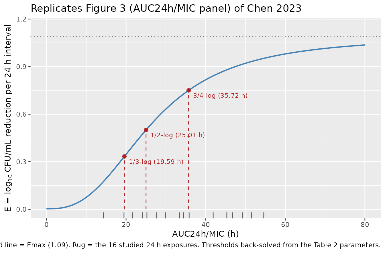
Replicate Figure 2: time-kill curves
Figure 2 of Chen 2023 shows the bacterial count in tissue-cage fluid
over the three-day dosing course and the follow-up period. The packaged
model reproduces the trajectory by integrating the per-interval
reduction; the untreated control arm is simulated by setting
AUC_TILM = 0, which collapses the sigmoid term and leaves
the near-zero control change E0 = 0.003.
sims <- bind_rows(
  simulate_arm(rep(0, 4), "Control (untreated)"),
  do.call(rbind, lapply(names(arm_auc), function(d) {
    simulate_arm(arm_auc[[d]], sprintf("%s mg/kg", d))
  }))
)
sims$arm <- factor(sims$arm,
                   levels = c("Control (untreated)",
                              sprintf("%s mg/kg", names(arm_auc))))

ggplot(sims, aes(time, log_cfu, colour = arm)) +
  geom_vline(xintercept = c(0, 24, 48), linetype = "dotted", colour = "grey65") +
  geom_hline(yintercept = 4, linetype = "dashed", colour = "grey40") +
  geom_line(linewidth = 0.8) +
  scale_x_continuous(breaks = seq(0, 96, by = 12)) +
  scale_y_continuous(breaks = seq(3, 8, by = 1)) +
  labs(x = "Time (h)",
       y = expression(log[10]~"CFU/mL"),
       colour = NULL,
       title = "Replicates Figure 2 of Chen 2023 (typical-value)",
       caption = paste("Dotted verticals = the three once-daily doses.",
                       "Dashed horizontal = 3-log10 reduction from the 10^7 CFU/mL baseline.")) +
  theme(legend.position = "bottom")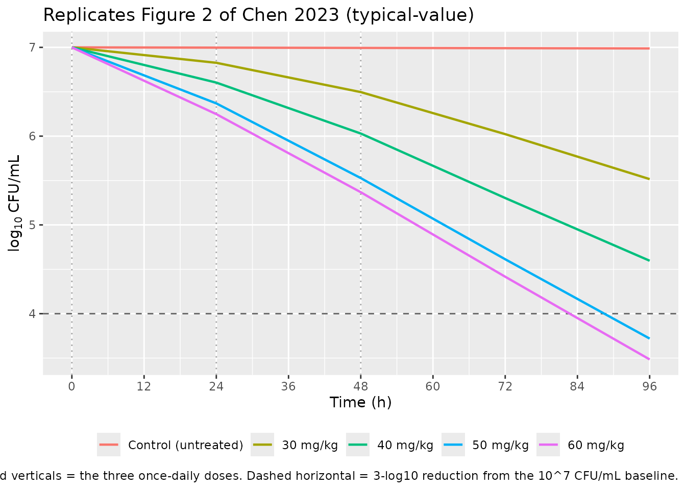
The simulated curves reproduce the qualitative findings of Section 3.3 and the Discussion: the 30 mg/kg arm falls well short of a 3-log10 reduction, the 50 and 60 mg/kg arms cross the bactericidal 3-log10 threshold, and the 50 and 60 mg/kg curves are nearly superimposed – the paper’s observation that the two highest doses were not significantly different because the maximum effect had already been reached at 50 mg/kg.
Because the exposures over the 24-48 h window after the final dose remain high (AUC24h/MIC of 46.8 h and 51.5 h at 50 and 60 mg/kg), the curves keep falling after dosing stops – the slow-elimination effect the Discussion highlights.
Validation: cumulative bacterial reduction
Section 3.3 reports the total reduction in bacterial count for each dose group. The Discussion states these accumulate “within 96 h after administration”, i.e. across four consecutive 24 h intervals: the three dosing intervals plus the 24-48 h window after the final dose. The comparison below uses exactly that window.
reported_total <- c(`30` = 1.48, `40` = 2.82, `50` = 3.39, `60` = 3.52)
reported_sd    <- c(`30` = 0.13, `40` = 0.10, `50` = 0.11, `60` = 0.15)

reduction_tbl <- do.call(rbind, lapply(names(arm_auc), function(d) {
  s <- simulate_arm(arm_auc[[d]], d)
  data.frame(
    dose      = as.integer(d),
    simulated = s$log_cfu[s$time == 0] - s$log_cfu[s$time == 96],
    reported  = reported_total[[d]],
    rep_sd    = reported_sd[[d]],
    stringsAsFactors = FALSE
  )
})) |>
  mutate(
    pct_diff = 100 * (simulated - reported) / reported,
    flag     = ifelse(abs(pct_diff) > 20, "*", "")
  )

reduction_tbl |>
  mutate(simulated = round(simulated, 3),
         reported  = sprintf("%.2f +/- %.2f", reported, rep_sd),
         pct_diff  = sprintf("%+.1f%%", pct_diff)) |>
  select(-rep_sd) |>
  rename("Dose (mg/kg)" = dose,
         "Simulated reduction at 96 h" = simulated,
         "Chen 2023 Section 3.3" = reported,
         "Difference" = pct_diff,
         ">20% flag" = flag) |>
knitr::kable(caption = "Cumulative log10 CFU/mL reduction over four 24 h intervals (0-96 h) versus the published totals.")| Dose (mg/kg) | Simulated reduction at 96 h | Chen 2023 Section 3.3 | Difference | >20% flag |
|---|---|---|---|---|
| 30 | 1.484 | 1.48 +/- 0.13 | +0.3% | |
| 40 | 2.404 | 2.82 +/- 0.10 | -14.8% | |
| 50 | 3.280 | 3.39 +/- 0.11 | -3.2% | |
| 60 | 3.515 | 3.52 +/- 0.15 | -0.1% |
Three of the four dose groups agree closely – 30 mg/kg (1.484 vs 1.48) and 60 mg/kg (3.516 vs 3.52) reproduce the published totals to within 0.01 log10, and 50 mg/kg agrees to 0.11 log10 (3.2%). No group exceeds the 20% flag threshold.
The 40 mg/kg group is the largest discrepancy: the model predicts 2.40 versus the reported 2.82 log10 (-14.8%). This is a property of the published parameters and exposures, not of the packaging – the Table 1 exposures for 40 mg/kg, pushed through the Table 2 sigmoid, cannot produce 2.82 log10. Note that the reported totals are not monotone in a way the exposures explain: the 30-to-40 mg/kg step in reported reduction (1.48 to 2.82, +1.34) is far larger than the 50-to-60 mg/kg step (3.39 to 3.52, +0.13), while the corresponding exposure increments are comparable. No parameter was tuned to close this gap.
Validation: PK/PD index thresholds
Table 2 also reports the AUC24h/MIC magnitude required
for a 1/3-log, 1/2-log and 3/4-log reduction per 24 h interval.
Back-solving those thresholds from the Table 2 parameters is a direct
internal-consistency check on the encoded equation.
threshold_tbl <- thresholds |>
  mutate(
    table2   = c(19.64, 33.45, 35.64),
    abstract = c(19.65, 23.86, 35.77),
    e_at_table2 = effect_of_index(table2)
  ) |>
  transmute(
    Reduction               = label,
    `Model-implied AUC24h/MIC (h)` = round(aucmic_h, 2),
    `Table 2 (h)`           = table2,
    `Abstract (h)`          = abstract,
    `E at the Table 2 value` = round(e_at_table2, 3),
    `Target E`              = round(effect, 3)
  )

knitr::kable(threshold_tbl,
caption = "Thresholds back-solved from the packaged Table 2 parameters versus the values printed in Chen 2023.")| Reduction | Model-implied AUC24h/MIC (h) | Table 2 (h) | Abstract (h) | E at the Table 2 value | Target E |
|---|---|---|---|---|---|
| 1/3-log | 19.59 | 19.64 | 19.65 | 0.335 | 0.333 |
| 1/2-log | 25.01 | 33.45 | 23.86 | 0.707 | 0.500 |
| 3/4-log | 35.72 | 35.64 | 35.77 | 0.749 | 0.750 |
The 1/3-log and 3/4-log thresholds are reproduced: the model implies 19.59 h and 35.72 h against printed values of 19.64 h and 35.64 h (Table 2) or 19.65 h and 35.77 h (Abstract) – agreement to 0.3% or better, which is what confirms both the equation’s printed form and the reduction-magnitude sign convention.
The 1/2-log threshold is internally inconsistent in the source. Substituting Table 2’s 33.45 h into Table 2’s own equation and parameters gives E = 0.707 log10 CFU/mL, i.e. very nearly a 3/4-log reduction rather than a 1/2-log one; the Abstract’s 23.86 h gives E = 0.466. The value consistent with the published parameters is 25.01 h. The packaged model encodes the four fitted parameters (which are self-consistent), so it necessarily disagrees with the printed 1/2-log threshold. This is recorded under Errata below; no parameter was adjusted.
Validation: encoding checks
PKNCA is not applicable to this model: there is no PK component and
no concentration observable to run non-compartmental analysis on. The
paper’s own PK analysis was non-compartmental and its outputs
(AUC0-24h, Cmax, T>MIC) are
inputs to the packaged model, reproduced verbatim in the
exposures table above rather than re-derived. In place of NCA, the
checks below verify that the ODE encoding faithfully implements the
published algebraic model.
# Check 1 -- interval-boundary exactness. The ODE must drop log10(bact) by
# exactly the algebraic E over each 24 h interval.
check1 <- do.call(rbind, lapply(names(arm_auc), function(d) {
  s   <- simulate_arm(arm_auc[[d]], d)
  b   <- s$log_cfu[s$time %in% c(0, 24, 48, 72, 96)]
  data.frame(dose = as.integer(d), interval = 1:4,
             ode_drop = -diff(b),
             algebraic = effect_of_index(arm_auc[[d]] / MIC))
})) |>
  mutate(abs_err = abs(ode_drop - algebraic))

# Check 2 -- untreated control. AUC_TILM = 0 must give a per-interval change
# of exactly E0 and leave the count essentially at the 10^7 CFU/mL baseline.
ctl <- simulate_arm(rep(0, 4), "control")
check2 <- c(per_interval_change = -diff(ctl$log_cfu[ctl$time %in% c(0, 24)]),
            e0_parameter = e0,
            log10_cfu_at_96h = ctl$log_cfu[ctl$time == 96])

# Check 3 -- saturation. As AUC_TILM grows without bound the per-interval
# reduction must approach Emax.
check3 <- c(reduction_at_huge_exposure =
              -diff(simulate_arm(rep(1e6, 4), "sat")$log_cfu[c(1, 49)]),
            emax_parameter = emax)

cat(sprintf("Check 1  max |ODE drop - algebraic E| over 16 intervals: %.3e\n",
            max(check1$abs_err)))
#> Check 1  max |ODE drop - algebraic E| over 16 intervals: 1.251e-04
cat(sprintf("Check 2  control per-interval change %.6f vs E0 %.6f; log10 CFU at 96 h = %.4f\n",
            check2[["per_interval_change"]], check2[["e0_parameter"]],
            check2[["log10_cfu_at_96h"]]))
#> Check 2  control per-interval change 0.003000 vs E0 0.003000; log10 CFU at 96 h = 6.9880
cat(sprintf("Check 3  reduction at saturating exposure %.6f vs Emax %.6f\n",
            check3[["reduction_at_huge_exposure"]], check3[["emax_parameter"]]))
#> Check 3  reduction at saturating exposure 1.089999 vs Emax 1.090000
check1 |>
  mutate(across(c(ode_drop, algebraic), ~ round(.x, 6)),
         abs_err = signif(abs_err, 3)) |>
  rename("Dose (mg/kg)" = dose, "24 h interval" = interval,
         "ODE log10 drop" = ode_drop, "Algebraic E" = algebraic,
         "|difference|" = abs_err) |>
knitr::kable(caption = "Check 1: the integrated ODE reproduces the algebraic per-interval reduction at every 24 h boundary, to solver tolerance.")| Dose (mg/kg) | 24 h interval | ODE log10 drop | Algebraic E | |difference| |
|---|---|---|---|---|
| 30 | 1 | 0.173852 | 0.173852 | 2.00e-07 |
| 30 | 2 | 0.329840 | 0.329840 | 1.00e-07 |
| 30 | 3 | 0.473749 | 0.473749 | 1.00e-07 |
| 30 | 4 | 0.506560 | 0.506561 | 9.00e-07 |
| 40 | 1 | 0.396627 | 0.396626 | 4.00e-07 |
| 40 | 2 | 0.573923 | 0.573923 | 3.00e-07 |
| 40 | 3 | 0.726610 | 0.726612 | 2.60e-06 |
| 40 | 4 | 0.706386 | 0.706395 | 8.40e-06 |
| 50 | 1 | 0.631114 | 0.631114 | 1.00e-07 |
| 50 | 2 | 0.841259 | 0.841260 | 1.00e-06 |
| 50 | 3 | 0.914606 | 0.914616 | 1.03e-05 |
| 50 | 4 | 0.893475 | 0.893547 | 7.21e-05 |
| 60 | 1 | 0.752065 | 0.752065 | 2.00e-07 |
| 60 | 2 | 0.879637 | 0.879639 | 1.70e-06 |
| 60 | 3 | 0.952012 | 0.952027 | 1.51e-05 |
| 60 | 4 | 0.931684 | 0.931809 | 1.25e-04 |
All three checks pass: the integrated trajectory matches the
algebraic per-interval model to solver tolerance, the untreated control
reproduces E0 and stays at the 10^7 CFU/mL baseline, and
saturating exposure drives the per-interval reduction to
Emax.
Dimensional analysis. AUC_TILM is in
ug*h/mL and mic in ug/mL, so
aucmic = AUC_TILM / mic has units of h – matching the
EC50 unit printed in Table 2 (“EC50 (h)”), which is itself
a useful confirmation that the index is AUC24h/MIC and not
a concentration ratio. kill_log10 is in log10 CFU/mL per 24
h interval, and dividing by 24 h before multiplying by
ln(10) * bact gives d/dt(bact) in
CFU/mL/h.
Assumptions and deviations
-
No PK model. Chen 2023 published no compartmental
PK model for tilmicosin in tissue-cage fluid (Section 2.5 states PK
parameters were computed with non-compartmental methods in WinNonlin
6.1). Drug exposure therefore enters the packaged model only through the
AUC_TILMcovariate. Simulating a regimen not in Table 1 requires an external source of per-interval AUC, for example a published tilmicosin popPK or PBPK model in swine; none was substituted here. - Within-interval uniformity of the kill rate. The published model is defined per 24 h interval, not as an instantaneous rate. The packaged ODE spreads each interval’s reduction uniformly across the interval. This is an encoding choice, not a published result; it is exact at every 24 h boundary (the only times Chen 2023 counted bacteria – Section 2.4), so no observed data point is affected, but the shape within an interval should not be interpreted as a paper finding. Check 1 above verifies the boundary exactness.
-
Only the AUC24h/MIC sub-model is packaged. Chen
2023 fitted the sigmoid to all three indices but reports parameter
values (Table 2) for
AUC24h/MIConly; forCmax/MICand%T>MICjust the R^2 values (0.90 and 0.83) are given. The other two sub-models are therefore not packaged, because theirE0,Emax,EC50andNare unpublished. No values were invented. -
No between-subject variability. Chen 2023 fitted
the PK/PD relationship by sigmoid regression across pooled tissue cages
and reported no random-effect variances, so the packaged model has no
etaparameters and is a typical-value model. The Table 1 standard deviations describe variability in the exposure inputs, not IIV on the PD parameters, and are not encoded as IIV. -
Residual SD fixed at zero. Only the coefficient of
determination (R^2 = 0.92) is reported for the fit; no residual standard
deviation is given.
addSd <- fixed(0)makes the model deterministic for typical-value simulation rather than encoding an invented error magnitude. -
Baseline count taken as exactly 10^7 CFU/mL.
Section 2.2 selected cages with “bacterial counts around 10^7 CFU/mL”
and Section 3.3 reports the untreated control “remained around 10^7
CFU/mL”. The packaged
log10_cfu0 <- fixed(7)adopts that nominal value; the paper gives no more precise mean baseline. -
MIC treated as a fixed model parameter. The MIC
(0.25 ug/mL) is a measured property of strain C44-15 rather than a
fitted parameter, and is wrapped in
fixed(). It is exposed as a parameter rather than hard-coded so the model can be applied to isolates of different susceptibility, which is the point of a PK/PD-index model. - Cumulative-reduction window inferred as 96 h. Section 3.3 reports total reductions without restating the window. The Discussion resolves it (“the number of bacteria could be reduced by 3 log10CFU/mL within 96 h after administration”), and the four-interval sum reproduces the 30 and 60 mg/kg totals to within 0.01 log10, which corroborates the 96 h reading.
Errata and internal inconsistencies in the source
No published erratum or corrigendum for this article was located. The following are internal inconsistencies within the article as published; none was resolved by adjusting a parameter.
-
The 1/2-log threshold is inconsistent with the paper’s own
parameters. Table 2 gives 33.45 h and the Abstract gives 23.86
h for the
AUC24h/MICneeded for a 1/2-log10 CFU/mL reduction. Substituted back into the Section 2.6 equation with the Table 2 parameters these give E = 0.707 and E = 0.466 respectively; the self-consistent value is 25.01 h. Table 2’s 33.45 h is the more serious of the two, corresponding to nearly a 3/4-log reduction and so almost duplicating the adjacent 3/4-log row (35.64 h). The 1/3-log and 3/4-log thresholds in both locations are consistent with the parameters to within 0.3%. - Abstract and Results disagree on all three thresholds. The Abstract reports 19.65 h, 23.86 h and 35.77 h; Section 3.4 and Table 2 report 19.64 h, 33.45 h and 35.64 h. For the 1/3-log and 3/4-log values the difference is negligible (and the Abstract’s 35.77 h is marginally closer to the model-implied 35.72 h than Table 2’s 35.64 h). Only the 1/2-log value differs materially, as above.
- The 40 mg/kg cumulative reduction is not reproducible from the published exposures and parameters (2.40 predicted versus 2.82 reported; -14.8%). The other three dose groups reproduce to within 3.2%. See the cumulative reduction section above.
-
Section 2.6 defines
Evia(Emax - E0), soEmaxis the effect at saturation, not the increment over baseline. This is stated only implicitly in the paper’s parameter descriptions (“Emax is the maximum antibacterial effect during the dosing interval”). The reading is confirmed by the reproduction of the 1/3-log and 3/4-log thresholds above; the alternative reading (E = E0 - Emax * ..., treatingEmaxas an increment) does not reproduce them.