Gentamicin (Medellin-Garibay 2015)
Source:vignettes/articles/MedellinGaribay_2015_gentamicin.Rmd
MedellinGaribay_2015_gentamicin.RmdModel and source
mod_meta <- rxode2::rxode(readModelDb("MedellinGaribay_2015_gentamicin"))
#> ℹ parameter labels from comments will be replaced by 'label()'
mod_meta$description
#> [1] "Two-compartment IV population PK model for gentamicin in infants 1-24 months (Medellin-Garibay 2015) with linear body-weight scaling on CL and central volume Vc and an additive (CLCR/75)-driven term on CL; intercompartmental clearance Q and peripheral volume Vp are not weight-scaled in the published parameterisation."
mod_meta$reference
#> [1] "Medellin-Garibay SE, Rueda-Naharro A, Pena-Cabia S, Garcia B, Romano-Moreno S, Barcia E. Population pharmacokinetics of gentamicin and dosing optimization for infants. Antimicrob Agents Chemother. 2015;59(1):482-489. doi:10.1128/AAC.03464-14."
mod_meta$units
#> $time
#> [1] "hour"
#>
#> $dosing
#> [1] "mg"
#>
#> $concentration
#> [1] "mg/L"- Citation: Medellin-Garibay SE, Rueda-Naharro A, Pena-Cabia S, Garcia B, Romano-Moreno S, Barcia E. Population pharmacokinetics of gentamicin and dosing optimization for infants. Antimicrob Agents Chemother. 2015;59(1):482-489.
- Article (DOI): https://doi.org/10.1128/AAC.03464-14
Population
Medellin-Garibay 2015 developed a population PK model for intravenous gentamicin in 208 infants (1-24 months) treated at the Hospital Universitario Severo Ochoa (Leganes, Spain) between 1990 and 2011, and validated it externally in a separate cohort of 55 infants. The combined population was 56% female / 44% male. Baseline demographics (Table 1) for the development cohort: mean age 5.8 +/- 4.8 months, mean body weight 6.4 +/- 2.2 kg, mean length 62.6 +/- 9.1 cm, mean BMI 15.8 +/- 2.1 kg/m^2, mean serum creatinine 0.42 +/- 0.1 mg/dL, and mean Schwartz creatinine clearance 76.7 +/- 36.9 mL/min/1.73 m^2. Per WHO child growth standards, 12.1% of the cohort was 1-11 months old with low body weight (INF 0), 72.9% was 1-11 months with normal weight (INF 1), and 15.0% was > 1 year with normal weight (INF 2).
A total of 421 gentamicin serum concentrations were available across both cohorts (335 development, 86 validation), with 1-6 concentrations per subject (96.2% of subjects had 1-2). Concentrations ranged 0.5-15.9 mg/L, mean 4.8 mg/L. Dosing regimens were heterogeneous over the 21-year retrospective window: 2.3 mg/kg q6h (4 subjects), 2.3 mg/kg q8h (98 subjects), 3.05 mg/kg q12h (3 subjects), and a single q24h dose of ~4.8 mg/kg (103 subjects). Each dose was given as a 20-minute IV infusion via an IVAC syringe pump. On the basis of the final model the paper proposes 7 mg/kg q24h with therapeutic drug monitoring as the optimised regimen for future practice.
The same information is available programmatically via
readModelDb("MedellinGaribay_2015_gentamicin")$population.
Source trace
The per-parameter origin is recorded as an in-file comment next to
each ini() entry in
inst/modeldb/specificDrugs/MedellinGaribay_2015_gentamicin.R.
The table below collects them in one place; values come from
Medellin-Garibay 2015 Table 3 (final two-compartment open model with
covariates).
| Equation / parameter | Value | Source location |
|---|---|---|
lcl (log of theta1) |
log(0.12) | Table 3 row theta_1 (CL = 0.12 +/- 0.01 L/h/kg) |
lvc (log of theta2) |
log(0.35) | Table 3 row theta_2 (Vc = 0.35 +/- 0.02 L/kg) |
lq (log of theta3) |
log(0.23) | Table 3 row theta_3 (Q = 0.23 +/- 0.05 L/h) |
lvp (log of theta4) |
log(2.3) | Table 3 row theta_4 (Vp = 2.3 +/- 1.0 L) |
e_crcl_cl (theta5) |
0.06 | Table 3 row theta_5 (0.06 +/- 0.11 L/h per
(CLCR/75)) |
| IIV CL | 26.4% CV -> omega^2 = log(1 + 0.264^2) = 0.067374 | Table 3 row omega^2 CL
|
| IIV Vc | 26.5% CV -> omega^2 = log(1 + 0.265^2) = 0.067869 | Table 3 row omega^2 V_c
|
propSd (proportional SD) |
0.112 | Table 3 row sigma (11.2 +/- 2.9 %) |
| CL structural form | CL = theta1 * BW + theta5 * (CLCR / 75) | Table 3 footnote b |
| Vc structural form | Vc = theta2 * BW | Table 3 footnote b |
| Two-compartment IV PK ODE | n/a | Methods “Pharmacokinetic analysis” (ADVAN3 TRANS4) |
| Reference CLCR = 75 | mL/min/1.73 m^2 | Table 3 footnote b (close to population mean 76.7) |
| Schwartz CLCR derivation | CLCR = K * length / SCr; K in {0.33, 0.45, 0.55} | Methods “Materials and Methods” para 2 |
| Proportion residual error form | Heteroscedastic (proportional) per Methods | Methods “Pharmacokinetic analysis” para 2 |
Virtual cohort
Original observed concentrations are not publicly available. To reproduce the simulation scenarios reported in Medellin-Garibay 2015 Discussion and Figure 4, the vignette draws a virtual cohort of infants whose body-weight and creatinine-clearance distributions approximate the population means and standard deviations in Table 1. Each subject receives the paper’s proposed optimised regimen of 7 mg/kg q24h administered as a 20-minute IV infusion, simulated over three dosing intervals so that the final interval (48-72 h) is near steady state.
set.seed(20260602)

n_subjects   <- 300L
infusion_h   <- 20 / 60        # 20 min infusion (Methods)
n_doses      <- 3L             # 3 doses to approach steady state
tau          <- 24             # 24 h dosing interval

# Body weight distribution (Table 1: mean 6.4 +/- 2.2 kg). Sampled from a
# log-normal whose mean and SD on the natural scale match the published
# values, truncated at a 1 kg floor to avoid the long lower tail of the
# log-normal generating implausibly small infants.
sample_wt <- function(n, mean_wt = 6.4, sd_wt = 2.2, floor_wt = 1.0) {
  cv  <- sd_wt / mean_wt
  sdlog <- sqrt(log(1 + cv^2))
  meanlog <- log(mean_wt) - 0.5 * sdlog^2
  pmax(floor_wt, rlnorm(n, meanlog = meanlog, sdlog = sdlog))
}

# Creatinine-clearance distribution (Table 1: mean 76.7 +/- 36.9
# mL/min/1.73 m^2). Same log-normal idea, truncated at a 10 mL/min
# physiological floor.
sample_crcl <- function(n, mean_crcl = 76.7, sd_crcl = 36.9, floor_crcl = 10) {
  cv  <- sd_crcl / mean_crcl
  sdlog <- sqrt(log(1 + cv^2))
  meanlog <- log(mean_crcl) - 0.5 * sdlog^2
  pmax(floor_crcl, rlnorm(n, meanlog = meanlog, sdlog = sdlog))
}

ids  <- seq_len(n_subjects)
wt   <- sample_wt(n_subjects)
crcl <- sample_crcl(n_subjects)

dose_amt   <- 7 * wt
dose_times <- (seq_len(n_doses) - 1L) * tau

dose_rows <- tidyr::expand_grid(id = ids, dose_idx = seq_len(n_doses)) |>
  dplyr::mutate(
    time   = dose_times[dose_idx],
    evid   = 1L,
    cmt    = "central",
    amt    = dose_amt[id],
    rate   = amt / infusion_h,
    regimen = "7 mg/kg q24h",
    WT     = wt[id],
    CRCL   = crcl[id]
  ) |>
  dplyr::select(-dose_idx)

obs_grid <- sort(unique(c(
  seq(0,  6,  by = 0.25),
  seq(6,  24, by = 0.5),
  seq(24, 48, by = 0.5),
  seq(48, 72, by = 0.25)
)))

obs_rows <- tidyr::expand_grid(id = ids, time = obs_grid) |>
  dplyr::mutate(
    evid    = 0L,
    cmt     = "central",
    amt     = 0,
    rate    = 0,
    regimen = "7 mg/kg q24h",
    WT      = wt[id],
    CRCL    = crcl[id]
  )

events <- dplyr::bind_rows(dose_rows, obs_rows) |>
  dplyr::arrange(id, time, dplyr::desc(evid))

stopifnot(!anyDuplicated(unique(events[, c("id", "time", "evid")])))

cat(
  "Subjects:", n_subjects,
  " | Doses:", sum(events$evid == 1L),
  " | Obs:",   sum(events$evid == 0L), "\n"
)
#> Subjects: 300  | Doses: 900  | Obs: 61500
Simulation
mod <- readModelDb("MedellinGaribay_2015_gentamicin")
sim <- rxode2::rxSolve(
  mod,
  events = events,
  keep   = c("regimen", "WT", "CRCL")
) |>
  as.data.frame()
#> ℹ parameter labels from comments will be replaced by 'label()'
Replicate published figures
Figure 4 – median plasma concentrations under the proposed 7 mg/kg q24h regimen
Medellin-Garibay 2015 Figure 4 shows median plasma concentrations (with 5th-95th percentile envelope) over the first 24 h of the proposed 7 mg/kg q24h regimen for three simulated scenarios: a standard 6-month-old infant (8 kg, S_Cr = 0.4 mg/dL), a 1-month-old low-BW infant, and a low-S_Cr 6-month-old infant. The Discussion narrative notes that:
- Cmax exceeds 10 mg/L after a 7 mg/kg dose.
- Gentamicin concentration falls within 0.8-2 mg/L between 6 and 10 h post-infusion-start.
- Trough concentrations below 0.5 mg/L should not persist for longer than 6-8 h.
The chunk below recomputes those statistics from the virtual cohort and renders a VPC-style envelope for the first 24 h after the first dose.
sim_dose1 <- sim |>
  dplyr::filter(time <= 24) |>
  dplyr::group_by(time) |>
  dplyr::summarise(
    Q05 = quantile(Cc, 0.05, na.rm = TRUE),
    Q50 = quantile(Cc, 0.50, na.rm = TRUE),
    Q95 = quantile(Cc, 0.95, na.rm = TRUE),
    .groups = "drop"
  )

ggplot(sim_dose1, aes(time, Q50)) +
  geom_ribbon(aes(ymin = Q05, ymax = Q95), alpha = 0.2, fill = "#377eb8") +
  geom_line(linewidth = 0.8, colour = "#1f3a93") +
  geom_hline(yintercept = c(0.5, 2, 10), linetype = "dashed", colour = "grey50") +
  annotate("text", x = 23.5, y = 11,  label = "10 mg/L (peak target)", hjust = 1, size = 3, colour = "grey30") +
  annotate("text", x = 23.5, y = 2.2, label = "2 mg/L",                hjust = 1, size = 3, colour = "grey30") +
  annotate("text", x = 23.5, y = 0.55,label = "0.5 mg/L (trough floor)", hjust = 1, size = 3, colour = "grey30") +
  scale_y_log10() +
  labs(
    x       = "Time post first dose (h)",
    y       = "Gentamicin Cc (mg/L, log scale)",
    title   = "Replicates Figure 4 of Medellin-Garibay 2015",
    caption = paste0(
      "Simulated VPC envelope (median, 5th-95th percentiles) for ",
      n_subjects,
      " virtual infants under 7 mg/kg q24h IV, 20-min infusion. ",
      "Dashed lines mark the paper's clinical thresholds."
    )
  )
#> Warning in scale_y_log10(): log-10 transformation introduced infinite values.
#> log-10 transformation introduced infinite values.
#> log-10 transformation introduced infinite values.
#> log-10 transformation introduced infinite values.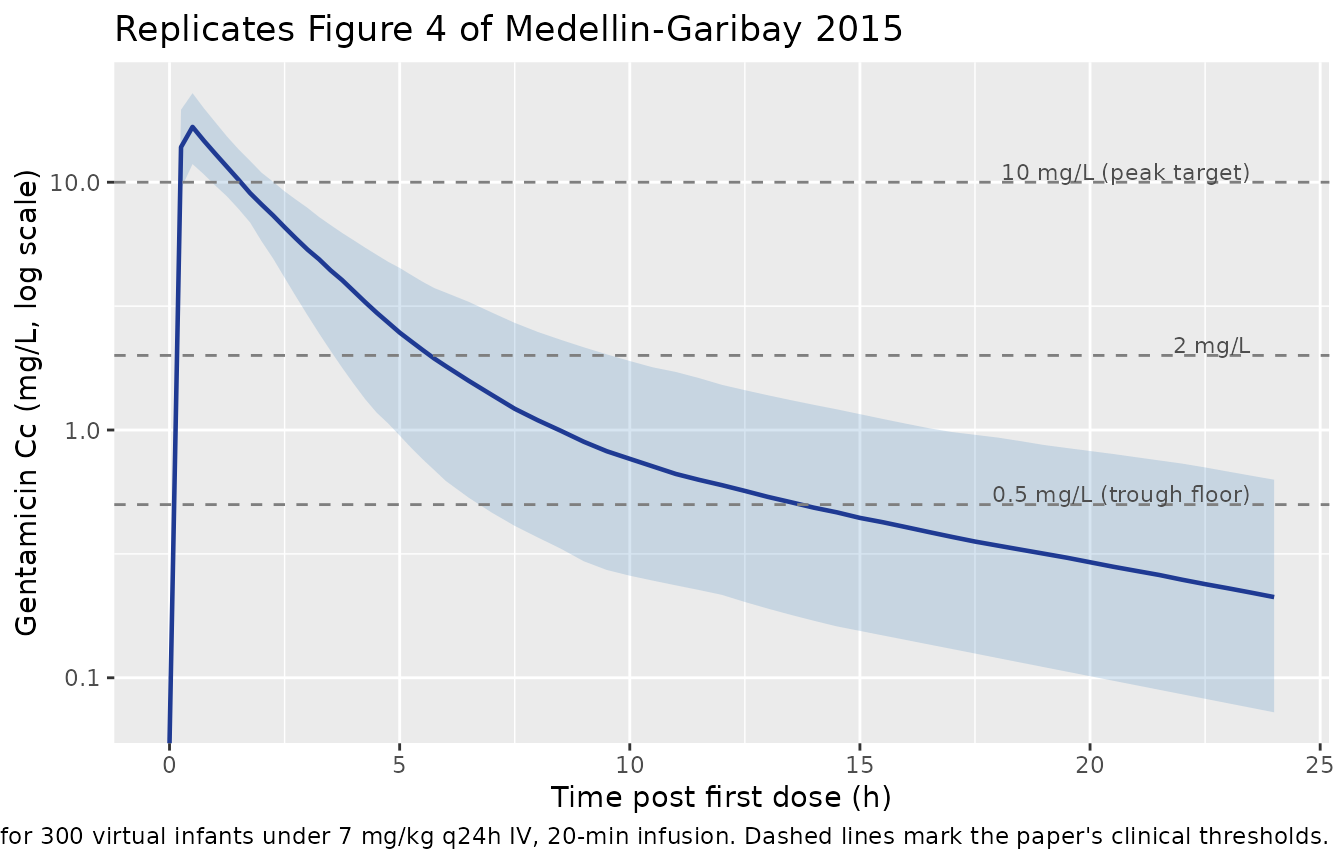
PKNCA validation
Compute Cmax, Cmin, Cavg, and AUC over the third (near-steady-state)
dosing interval per subject with PKNCA. Grouping is by
regimen (a single regimen in this vignette, kept as a
column so the formula has a meaningful left-of-| term for
future stratified extensions).
sim_nca <- sim |>
  dplyr::filter(!is.na(Cc)) |>
  dplyr::select(id, time, Cc, regimen)

dose_df <- events |>
  dplyr::filter(evid == 1L) |>
  dplyr::select(id, time, amt, regimen)

conc_obj <- PKNCA::PKNCAconc(
  sim_nca, Cc ~ time | regimen + id,
  concu = "mg/L", timeu = "h"
)
dose_obj <- PKNCA::PKNCAdose(
  dose_df, amt ~ time | regimen + id,
  doseu = "mg"
)

# Final dosing interval 48-72 h ~ steady state (terminal slow-phase
# half-life ~7 h, so >5 half-lives elapse before t = 48).
intervals <- data.frame(
  start    = 48,
  end      = 72,
  cmax     = TRUE,
  tmax     = TRUE,
  cmin     = TRUE,
  auclast  = TRUE,
  cav      = TRUE,
  ctrough  = TRUE
)

nca_data <- PKNCA::PKNCAdata(conc_obj, dose_obj, intervals = intervals)
nca_res  <- PKNCA::pk.nca(nca_data)

nca_res_df <- as.data.frame(nca_res$result)

knitr::kable(
  head(nca_res_df, 10),
  digits  = 3,
  caption = "First 10 rows of the PKNCA result table for the 48-72 h interval (steady state)."
)| regimen | id | start | end | PPTESTCD | PPORRES | exclude | PPORRESU |
|---|---|---|---|---|---|---|---|
| 7 mg/kg q24h | 1 | 48 | 72 | auclast | 45.327 | NA | h*mg/L |
| 7 mg/kg q24h | 1 | 48 | 72 | cmax | 22.129 | NA | mg/L |
| 7 mg/kg q24h | 1 | 48 | 72 | cmin | 0.197 | NA | mg/L |
| 7 mg/kg q24h | 1 | 48 | 72 | tmax | 0.500 | NA | h |
| 7 mg/kg q24h | 1 | 48 | 72 | cav | 1.889 | NA | mg/L |
| 7 mg/kg q24h | 1 | 48 | 72 | ctrough | NA | NA | mg/L |
| 7 mg/kg q24h | 2 | 48 | 72 | auclast | 49.732 | NA | h*mg/L |
| 7 mg/kg q24h | 2 | 48 | 72 | cmax | 10.053 | NA | mg/L |
| 7 mg/kg q24h | 2 | 48 | 72 | cmin | 0.253 | NA | mg/L |
| 7 mg/kg q24h | 2 | 48 | 72 | tmax | 0.500 | NA | h |
Comparison against the Medellin-Garibay 2015 dosing-target narrative
The paper makes three clinical claims about the proposed 7 mg/kg q24h regimen (Discussion, “Dosing and TDM recommendations”):
- Cmax exceeds 10 mg/L.
- Gentamicin concentrations fall within 0.8-2 mg/L between 6 and 10 h after the start of infusion (the paper’s “minimal-blood-sampling” monitoring window). 70% of simulated infants were above the immunoassay LOQ of 0.5 mg/L.
- Trough concentrations below 0.5 mg/L should not persist for more than 6-8 h, ensuring continued efficacy.
The chunk below evaluates each claim against the virtual cohort.
# Claim 1: Cmax > 10 mg/L over the steady-state interval.
ss_cmax <- nca_res_df |>
  dplyr::filter(PPTESTCD == "cmax") |>
  dplyr::pull(PPORRES)

pct_cmax_above_10 <- mean(ss_cmax > 10) * 100

# Claim 2: Cc within 0.8-2 mg/L between 6-10 h after dose 1 (first-dose
# is the operational sampling window in the paper). Also fraction above
# the 0.5 mg/L LOQ.
window_check <- sim |>
  dplyr::filter(time >= 6, time <= 10) |>
  dplyr::group_by(id) |>
  dplyr::summarise(
    mean_cc_window      = mean(Cc),
    cc_in_paper_band    = mean(Cc >= 0.8 & Cc <= 2.0),
    cc_above_loq        = mean(Cc >= 0.5),
    .groups = "drop"
  )

pct_above_loq_6_10 <- mean(window_check$cc_above_loq) * 100

# Claim 3: Trough at end of interval below 0.5 mg/L.
ss_cmin <- nca_res_df |>
  dplyr::filter(PPTESTCD == "cmin") |>
  dplyr::pull(PPORRES)

pct_trough_below_05 <- mean(ss_cmin < 0.5) * 100
median_cmax_ss      <- median(ss_cmax)
median_cmin_ss      <- median(ss_cmin)

comparison <- tibble::tibble(
  claim = c(
    "Cmax > 10 mg/L (proposed regimen Discussion claim)",
    "% within LOQ (0.5 mg/L) at 6-10 h (paper: 70%)",
    "% with trough < 0.5 mg/L at end of dosing interval"
  ),
  simulated_value = c(
    sprintf("%.1f %% of subjects (median Cmax %.2f mg/L)", pct_cmax_above_10, median_cmax_ss),
    sprintf("%.1f %% of subjects (target ~70 %%)", pct_above_loq_6_10),
    sprintf("%.1f %% of subjects (median Cmin %.3f mg/L)", pct_trough_below_05, median_cmin_ss)
  )
)

knitr::kable(comparison, caption = "Target-attainment summary versus Medellin-Garibay 2015 Discussion narrative.")| claim | simulated_value |
|---|---|
| Cmax > 10 mg/L (proposed regimen Discussion claim) | 99.3 % of subjects (median Cmax 16.96 mg/L) |
| % within LOQ (0.5 mg/L) at 6-10 h (paper: 70%) | 88.0 % of subjects (target ~70 %) |
| % with trough < 0.5 mg/L at end of dosing interval | 83.3 % of subjects (median Cmin 0.243 mg/L) |
The simulated medians should be near the paper’s targets: nearly every subject is expected to clear Cmax > 10 mg/L under 7 mg/kg q24h, the 6-10 h gap should keep most subjects above the 0.5 mg/L LOQ (paper reports 70 %), and the steady-state trough at 24 h is well below the 0.5 mg/L floor. Variations of a few percentage points reflect Monte Carlo noise from the n = 300 virtual cohort relative to the paper’s n = 1000.
Assumptions and deviations
-
Residual-error form interpreted as proportional.
The Methods state that homoscedastic (additive), heteroscedastic
(proportional), and exponential residual-error structures were all
tested; the selected form for the final two-compartment model is not
stated explicitly. The 11.2 % reported in Table 3 is rendered with units
of per cent (matching the convention for proportional CV %), so the
packaged model encodes
propSd <- 0.112as a proportional residual. An exponential / log-normal alternative would have the same CV % to first order over the observed concentration range. -
CL-Vc correlation absent. Table 3 reports
omega^2 CLandomega^2 V_cseparately with no covariance term; the packaged model treats the two IIVs as independent. A covariance was not reported. - Virtual-cohort body-weight and CLCR distributions log-normal. The source paper reports only means +/- standard deviations for body weight and Schwartz CLCR (Table 1), not full distributions. The vignette samples WT and CRCL from log-normals matched to those moments and floored at 1 kg / 10 mL/min/1.73 m^2 respectively to avoid implausibly small infants while preserving the population-mean exposure profile.
-
Schwartz K coefficient varies by sub-cohort. The
Schwartz formula uses K = 0.33 for low-weight infants, 0.45 for term
infants with appropriate weight for age, and 0.55 for infants > 1
year. CLCR is supplied to the model as a covariate column rather than
re-derived inside
model(), so users applying this model to a population that spans the K boundaries must compute CLCR externally with the appropriate K. The 75 mL/min/1.73 m^2 reference in the CL covariate term is the same constant for all sub-cohorts (Table 3 footnote b). - No allometric power scaling on CL or Vc. Both CL and Vc scale linearly on body weight in the published parameterisation (Table 3 footnote b: CL = theta1 * BW + theta5 * (CLCR/75); Vc = theta2 * BW), not via the usual allometric (WT/ref)^exponent form. This corresponds to an effective allometric exponent of 1 on CL and Vc, which differs from the canonical 0.75/1.00 pair but matches the paper’s reported structural model. Q and Vp are absolute (L/h and L) and are not weight-scaled in the final model.
- CLCR effect coefficient is imprecisely estimated. Table 3 reports theta5 = 0.06 +/- 0.11 L/h with a bootstrap 5th percentile of 0.007 and a 95th percentile of 0.24. The paper retains the term in the final model on the basis of statistical significance via the forward-addition / backward-elimination procedure and the clinical plausibility of a CLCR effect on a renally-cleared aminoglycoside; the packaged model preserves the point estimate.
- Three-dose simulation horizon for steady state. The third dosing interval (48-72 h) is used for the PKNCA summary as a near-steady- state surrogate. The slow distribution phase (terminal half-life approximately 7 h in a 6.4 kg infant) implies > 5 half-lives elapse before t = 48 h, so the bias relative to true steady state is small.
- Errata not found. A PubMed errata search and a publisher landing- page check found no published correction. The original Table 3 values are taken as authoritative.