Naloxone (Al Yacoub 2025)
Source:vignettes/articles/AlYacoub_2025_naloxone.Rmd
AlYacoub_2025_naloxone.RmdModel and source
- Citation: Al Yacoub ON, Cheng S, Fayed MS, Fisher J, Brooks J, Seaquist E, Kumar A, Moheet A, Eberly LE, Coles LD. Intranasal Naloxone During Recurrent Exercise in Individuals with Type-1 Diabetes Mellitus: Evaluation of the Clinical Predictors of Pharmacokinetics and Exposure-Response. J Clin Pharmacol. 2025;65:1577-1586. doi:10.1002/jcph.70067
- Description: Two-compartment population PK model for intranasal naloxone (4 mg Narcan nasal spray, four doses at 0, 45, 300 and 345 min) in adults with type 1 diabetes mellitus during recurrent exercise (Al Yacoub 2025): sequential zero-order input into the depot over D1 followed by first-order absorption into the central compartment, linear elimination, apparent clearances and volumes allometrically scaled by body weight (fixed exponents 0.75 and 1, reference 70 kg), between-subject variability on CL/F, V1/F and D1, and combined proportional and additive residual error. Time unit is minutes.
- Article: https://doi.org/10.1002/jcph.70067 (open access; the NONMEM control stream of the final model is in the Supporting Information)
Al Yacoub 2025 is the PK arm of a crossover trial testing whether intranasal (IN) naloxone given during exercise preserves the counterregulatory response to a hypoglycemic clamp the next day in people with type 1 diabetes. On the naloxone day each participant received four 4 mg Narcan nasal-spray doses, at the start of a 90-min morning exercise bout (0 min), 45 min into it, and again at the start of and 45 min into an afternoon bout (300 and 345 min). The final model is a two-compartment model in which each IN dose enters the depot as a zero-order input of duration D1 and is then absorbed first-order into the central compartment (Figure 3). All parameters are apparent (CL/F, V1/F, …) and the time unit is minutes.
Population
27 adults with type 1 diabetes and intact awareness of hypoglycemia contributed 271 plasma naloxone concentrations (Table 1): 11 women and 16 men, age 29.8 +/- 9.2 years, BMI 26.5 +/- 4.3 kg/m^2, HbA1c 6.9 +/- 0.8%, diabetes duration 16 +/- 7.9 years. One further participant was excluded because the model did not converge with their data. Body weight, the only covariate, is not tabulated. Race and ethnicity are not reported. The study was single centre (University of Minnesota, USA). During the PK day euglycemia was maintained with insulin and a variable-rate glucose infusion.
The same information is available programmatically via
readModelDb("AlYacoub_2025_naloxone")()$population.
Source trace
Every ini() value carries an in-file comment in
inst/modeldb/specificDrugs/AlYacoub_2025_naloxone.R.
| Equation / parameter | Value | Source location |
|---|---|---|
lka |
log(0.0272 1/min) | Table 2 ‘KA (per min)’; THETA(1) |
lcl (CL/F at 70 kg) |
log(6.82 L/min) | Table 2 ‘CL/F (L/min/70 kg)’; THETA(2) |
lvc (V1/F at 70 kg) |
log(171 L) | Table 2 ‘V1/F (L/70 kg)’; THETA(3) |
lq (Q/F at 70 kg) |
log(2.97 L/min) | Table 2 ‘CL2/F (L/min/70 kg)’; THETA(4) |
lvp (V2/F at 70 kg) |
log(278 L) | Table 2 ‘V2/F (L/70 kg)’; THETA(5) |
ld1 (zero-order input duration) |
log(7.33 min) | Table 2 ‘D1 (min)’; THETA(6) |
e_wt_cl, e_wt_vc
|
0.75, 1 (fixed) | Results ‘Population PK Analysis’ equations and text; supplement code |
etalcl, etalvc, etald1
|
0.103, 0.268, 0.108 | Table 2 BSV column (variances; CV 32.9%, 55.4%, 33.8%) |
propSd |
0.237 | Table 2 ‘RUV% (proportional)’ 5.62 = sigma^2 0.0562; ‘RUV CV%’ 23.7 |
addSd |
0.348 ng/mL | Table 2 ‘RUV (ng/mL)’ 0.121 = sigma^2; ‘RUV CV%’ 34.8 |
CL, Q (WT/70)^0.75; V1, V2 (WT/70)^1
|
n/a | Results equations; supplement
TVCL = THETA(2)*(WT/70)**0.75,
TVV2 = THETA(3)*(WT/70)
|
| Zero-order input into depot then first-order absorption | n/a | Results; Figure 3; supplement ADVAN4 TRANS4 with
D1, RATE in $INPUT
|
| Two-compartment linear disposition | n/a | Results; Figure 3; supplement ADVAN4 TRANS4
|
Cc ~ add(addSd) + prop(propSd) |
n/a | Results RUV equation; supplement
Y = F + EPS(1)*IPRED + EPS(2)
|
Typical-value checks
Each IN dose goes into depot with
rate = -2, so it enters the depot at a constant rate over
the modelled duration D1 before first-order absorption. The
paper reports the elimination half-life, 0.693 / beta, as a
secondary parameter of 99.1 min (Table 2). The closed form for a 70-kg
participant reproduces it from the five disposition estimates:
k10 <- 6.82 / 171
k12 <- 2.97 / 171
k21 <- 2.97 / 278
s <- k10 + k12 + k21
beta <- (s - sqrt(s^2 - 4 * k10 * k21)) / 2
t_half_beta <- log(2) / beta
t_half_beta
#> [1] 99.1407
stopifnot(abs(t_half_beta - 99.1) < 0.1)
The abstract gives the intercompartmental clearance as “2.97 L/h/70 kg”; Table 2 gives L/min. Only the per-minute reading reproduces the 99.1 min half-life, so the model uses L/min.
mod <- readModelDb("AlYacoub_2025_naloxone")
mod_typ <- rxode2::zeroRe(mod)
#> ℹ parameter labels from comments will be replaced by 'label()'

dose_times <- c(0, 45, 300, 345)
obs_grid <- sort(unique(c(seq(0, 1440, by = 2.5), 295, 415)))

make_events <- function(id, wt, grid = obs_grid) {
  bind_rows(
    tibble(
      id = id,
      time = dose_times,
      evid = 1L,
      amt = 4,
      rate = -2,
      cmt = "depot"
    ),
    tibble(id = id, time = grid, evid = 0L, amt = 0, rate = 0, cmt = "central")
  ) |>
    mutate(WT = wt) |>
    arrange(id, time, desc(evid))
}

sim_typ <- rxode2::rxSolve(
  mod_typ,
  events = make_events(1L, 70),
  rtol = 1e-10,
  atol = 1e-12
) |>
  as.data.frame()
#> ℹ omega/sigma items treated as zero: 'etalcl', 'etalvc', 'etald1'

ggplot(sim_typ |> filter(time <= 600), aes(time, Cc)) +
  geom_line() +
  geom_vline(xintercept = dose_times, linetype = "dotted", colour = "grey40") +
  labs(
    x = "Time (min)",
    y = "Naloxone Cc (ng/mL)",
    title = "Typical 70-kg participant, four 4 mg intranasal doses",
    caption = "Dotted lines: dose times (0, 45, 300, 345 min)."
  )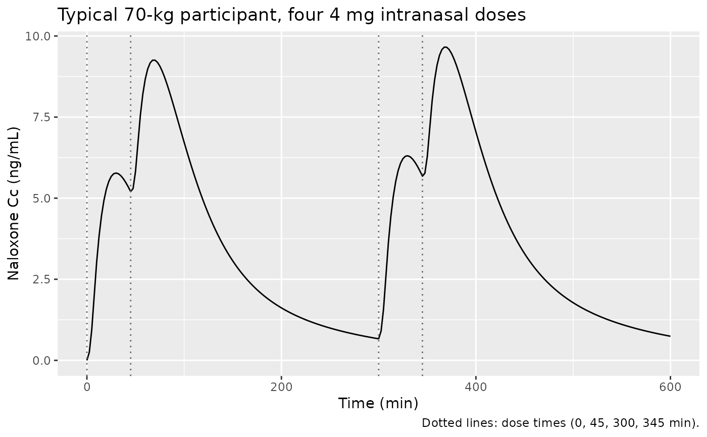
The total AUC of the typical profile must equal the total dose over CL/F (4 x 4 mg / 6.82 L/min, x1000 for ng/mL); integrating the 1440-min solve captures all but the unabsorbed and still-circulating remainder.
auc_trap <- function(t, y) sum(diff(t) * (head(y, -1) + tail(y, -1)) / 2)
last <- sim_typ[nrow(sim_typ), ]
auc_obs <- auc_trap(sim_typ$time, sim_typ$Cc)
# Remaining amount in the body at 1440 min, cleared at CL/F after the window.
auc_remaining <- (last$depot + last$central + last$peripheral1) / 6.82 * 1000
auc_expected <- 16 / 6.82 * 1000
c(auc_window = auc_obs, auc_total = auc_obs + auc_remaining, expected = auc_expected)
#> auc_window  auc_total   expected
#>   2345.775   2346.066   2346.041
stopifnot(abs((auc_obs + auc_remaining) / auc_expected - 1) < 0.01)
Virtual cohort
Body weight is not reported, so the maintainers derived it from the Table 1 BMI distribution (normal, 26.5 +/- 4.3 kg/m^2, truncated to 18-40) and an assumed sex-specific height (normal; women 1.63 +/- 0.07 m, men 1.77 +/- 0.075 m, approximate US adult values), with the Table 1 sex split (11 of 27 female). 200 virtual participants receive the four-dose IN regimen.
rxode2::rxSetSeed(2025)
n_sub <- 200
cohort <- tibble(
  id = seq_len(n_sub),
  female = rbinom(n_sub, 1, 11 / 27),
  height = ifelse(female == 1, rnorm(n_sub, 1.63, 0.07), rnorm(n_sub, 1.77, 0.075)),
  bmi = pmin(pmax(rnorm(n_sub, 26.5, 4.3), 18), 40)
) |>
  mutate(WT = bmi * height^2)

summary(cohort$WT)
#>    Min. 1st Qu.  Median    Mean 3rd Qu.    Max.
#>   42.18   65.13   76.17   76.76   87.05  119.57

vpc_grid <- sort(unique(c(seq(0, 600, by = 5), 295, 415)))
ev_pop <- bind_rows(lapply(seq_len(n_sub), function(i) {
  make_events(i, cohort$WT[i], grid = vpc_grid)
})) |>
  mutate(treatment = "Naloxone 4 mg IN x 4")

sim_pop <- rxode2::rxSolve(mod, events = ev_pop, keep = "treatment") |>
  as.data.frame()
#> ℹ parameter labels from comments will be replaced by 'label()'
Replicate Figure 5 (VPC)
Figure 5 is a VPC over the day-1 samples (-5, 5, 15, 30, 60, 120, 295, 310, 325, 355, 385 and 415 min), with bins whose edges are the orange ticks on the x-axis (about 0, 22, 45, 90, 207, 305, 318, 340, 370, 400 and 430 min). The first bin pools the 5- and 15-min samples. The observed medians below were read off Figure 5 by the maintainers and are approximate (+/- 0.3 ng/mL).
sample_times <- c(5, 15, 30, 60, 120, 295, 310, 325, 355, 385, 415)
bin_of <- function(t) {
  cut(t, c(0, 22, 45, 90, 207, 305, 318, 340, 370, 400, 430), right = FALSE)
}

fig5_obs <- tibble(
  bin_time = c(15, 30, 60, 120, 295, 310, 325, 355, 385, 415),
  obs_median = c(2.0, 5.0, 7.6, 4.9, 0.6, 3.6, 5.7, 7.3, 7.4, 4.4)
) |>
  mutate(bin = bin_of(bin_time))

sim_samples <- sim_pop |>
  filter(time %in% sample_times) |>
  mutate(bin = bin_of(time))

# One simulated "observation" per sample: IPRED plus residual error drawn at
# the Table 2 SDs (the VPC is of observations, not of IPRED).
rxode2::rxSetSeed(2026)
sim_samples <- sim_samples |>
  mutate(
    dv = Cc * (1 + rnorm(n(), 0, 0.237)) + rnorm(n(), 0, 0.348)
  )

vpc_sim <- sim_samples |>
  group_by(bin) |>
  summarise(
    p05 = quantile(dv, 0.05),
    p50 = median(dv),
    p95 = quantile(dv, 0.95),
    .groups = "drop"
  ) |>
  left_join(fig5_obs, by = "bin") |>
  mutate(pct_diff = 100 * (p50 - obs_median) / obs_median)

vpc_sim |>
  select(bin_time, p05, p50, p95, obs_median, pct_diff) |>
  dplyr::rename(
    "Bin (plotted time, min)" = bin_time,
    "Sim 5th pct (ng/mL)" = p05,
    "Sim median (ng/mL)" = p50,
    "Sim 95th pct (ng/mL)" = p95,
    "Figure 5 observed median (ng/mL)" = obs_median,
    "% diff (median)" = pct_diff
  ) |>
knitr::kable(digits = 2, caption = "Binned simulated percentiles vs the Figure 5 observed medians.")| Bin (plotted time, min) | Sim 5th pct (ng/mL) | Sim median (ng/mL) | Sim 95th pct (ng/mL) | Figure 5 observed median (ng/mL) | % diff (median) |
|---|---|---|---|---|---|
| 15 | 0.25 | 1.83 | 6.98 | 2.0 | -8.74 |
| 30 | 2.60 | 5.05 | 9.60 | 5.0 | 1.07 |
| 60 | 4.10 | 7.26 | 13.79 | 7.6 | -4.52 |
| 120 | 2.02 | 4.67 | 8.39 | 4.9 | -4.60 |
| 295 | -0.14 | 0.82 | 2.34 | 0.6 | 36.66 |
| 310 | 1.46 | 3.32 | 6.91 | 3.6 | -7.89 |
| 325 | 2.62 | 5.54 | 9.51 | 5.7 | -2.76 |
| 355 | 3.85 | 7.04 | 12.71 | 7.3 | -3.55 |
| 385 | 3.76 | 7.98 | 14.17 | 7.4 | 7.77 |
| 415 | 2.18 | 5.41 | 10.65 | 4.4 | 22.88 |
ggplot(vpc_sim, aes(bin_time)) +
  geom_ribbon(aes(ymin = p05, ymax = p95), fill = "lightblue", alpha = 0.5) +
  geom_line(aes(y = p50)) +
  geom_point(aes(y = obs_median), shape = 21, size = 2.5, fill = "white") +
  labs(
    x = "Time (min)",
    y = "Naloxone concentration (ng/mL)",
    title = "Replicates Figure 5 of Al Yacoub 2025",
    caption = paste(
      "Line and band: simulated median and 5th-95th percentiles per Figure 5 bin.",
      "Open circles: Figure 5 observed medians (digitised).",
      sep = "\n"
    )
  )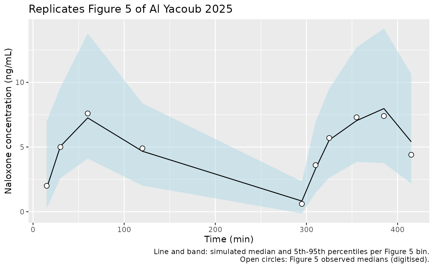
The trough bin at 295 min sits near 0.6 ng/mL, where a 0.2 ng/mL reading error is a third of the value, so it is left out of the agreement check.
PKNCA
Per-participant Cmax and AUC0-600 (the exposure metrics of the paper’s exposure-response analysis, there called AUCall) and the terminal half-life after the last dose, computed with PKNCA on the simulated IPRED profiles.
nca_conc <- sim_pop |>
  filter(!is.na(Cc)) |>
  select(id, time, Cc, treatment)
nca_dose <- ev_pop |>
  filter(evid == 1) |>
  select(id, time, amt, treatment)

conc_obj <- PKNCA::PKNCAconc(nca_conc, Cc ~ time | treatment + id)
dose_obj <- PKNCA::PKNCAdose(nca_dose, amt ~ time | treatment + id)
intervals <- data.frame(
  start = 0,
  end = 600,
  cmax = TRUE,
  tmax = TRUE,
  auclast = TRUE
)
nca_res <- PKNCA::pk.nca(PKNCA::PKNCAdata(conc_obj, dose_obj, intervals = intervals))

nca_summary <- as.data.frame(nca_res) |>
  filter(PPTESTCD %in% c("cmax", "tmax", "auclast")) |>
  group_by(treatment, PPTESTCD) |>
  summarise(
    median = median(PPORRES),
    p05 = quantile(PPORRES, 0.05),
    p95 = quantile(PPORRES, 0.95),
    .groups = "drop"
  )
nca_summary |>
  dplyr::rename(
    "Treatment" = treatment,
    "PKNCA parameter" = PPTESTCD,
    "Median" = median,
    "5th pct" = p05,
    "95th pct" = p95
  ) |>
knitr::kable(digits = 2, caption = "Simulated per-participant NCA over 0-600 min (Cmax ng/mL, Tmax min, AUC ng*min/mL).")| Treatment | PKNCA parameter | Median | 5th pct | 95th pct |
|---|---|---|---|---|
| Naloxone 4 mg IN x 4 | auclast | 2177.22 | 1168.08 | 3700.38 |
| Naloxone 4 mg IN x 4 | cmax | 9.01 | 5.41 | 14.76 |
| Naloxone 4 mg IN x 4 | tmax | 370.00 | 360.00 | 380.00 |
The Discussion reports observed peak concentrations after the four doses of about 2.5 to 15 ng/mL; the simulated 5th-95th percentile range of Cmax is 5.4 to 14.8 ng/mL.
The terminal half-life of a typical 70-kg participant, from the 24-h typical-value solve, is compared with the Table 2 value:
typ_conc <- sim_typ |>
  filter(!is.na(Cc)) |>
  # A single-subject solve returns no id column.
  mutate(id = 1L, treatment = "Naloxone 4 mg IN x 4") |>
  select(id, time, Cc, treatment)
typ_dose <- tibble(id = 1L, time = dose_times, amt = 4, treatment = "Naloxone 4 mg IN x 4")
typ_nca <- PKNCA::pk.nca(PKNCA::PKNCAdata(
  PKNCA::PKNCAconc(typ_conc, Cc ~ time | treatment + id),
  PKNCA::PKNCAdose(typ_dose, amt ~ time | treatment + id),
  intervals = data.frame(start = 345, end = 1440, half.life = TRUE)
))

hl_tbl <- nlmixr2lib::ncaComparisonTable(
  simulated = typ_nca,
  reference = data.frame(treatment = "Naloxone 4 mg IN x 4", half.life = 99.1),
  by = "treatment",
  params = "half.life",
  units = c(half.life = "min")
)
knitr::kable(hl_tbl, caption = "Terminal half-life, typical 70-kg participant.")| NCA parameter | treatment | Reference | Simulated | % diff |
|---|---|---|---|---|
| t½ (min) | Naloxone 4 mg IN x 4 | 99.1 | 98.5 | -0.6% |
hl_sim <- as.data.frame(typ_nca) |>
  filter(PPTESTCD == "half.life") |>
  pull(PPORRES)
stopifnot(abs(hl_sim / 99.1 - 1) < 0.02)
Assumptions and deviations
- Body weight of the virtual cohort. Not reported; derived from the Table 1 BMI distribution and assumed sex-specific heights (see Virtual cohort). The simulated median weight is about 77 kg.
-
Residual-error magnitudes. Table 2 reports the
proportional term as “RUV% 5.62” and the additive term as “0.121 ng/mL”,
with a “RUV CV%” column of 23.7 and 34.8 computed as sqrt(sigma^2)
(footnote c). The supplement’s
$ERROR(Y = F + EPS(1)*IPRED + EPS(2)) makes the estimates SIGMA variances, so the model carries the SDs:propSd= 0.237 andaddSd= sqrt(0.121) = 0.348 ng/mL. - Units of the intercompartmental clearance. The abstract states “2.97 L/h/70 kg”; Table 2 states L/min. The model uses L/min, the only reading consistent with the reported 99.1 min half-life (checked above).
- Diabetes duration. The abstract gives an eligibility range of 2-20 years and the Methods 2-30 years; this does not enter the model.
- Figure 5 values were read off the published figure by the maintainers and are approximate. The VPC here bins at the paper’s bin edges but uses nominal sample times and simulated weights, so small differences from Figure 5 are expected.
- No exposure-response model. The paper’s exposure-response analysis was a set of linear regressions with no significant relationship, so no PD component is included.