Pevonedistat (Faessel 2019)
Source:vignettes/articles/Faessel_2019_pevonedistat.Rmd
Faessel_2019_pevonedistat.RmdModel and source
- Citation: Faessel HM, Mould DR, Zhou X, Faller DV, Sedarati F, Venkatakrishnan K. Population pharmacokinetics of pevonedistat alone or in combination with standard of care in patients with solid tumours or haematological malignancies. Br J Clin Pharmacol. 2019;85(11):2568-2579. doi:10.1111/bcp.14078
- Description: Two-compartment population PK model for intravenous pevonedistat (TAK-924, MLN4924) in adults with solid tumours or haematological malignancies, with body-surface-area scaling of clearance and volumes, an albumin effect on distributional clearance, and reduced clearance on concomitant carboplatin plus paclitaxel
- Article: https://doi.org/10.1111/bcp.14078
- Supplement: Supplementary Figure S1 (goodness-of-fit plots only; it contains no parameter values and no control stream).
Pevonedistat (TAK-924, formerly MLN4924) is a first-in-class small-molecule NEDD8-activating enzyme inhibitor given as a 1-hour intravenous infusion. Faessel 2019 pooled six phase I / Ib dose-escalation studies into a single two-compartment population PK model with linear elimination.
Population
Six clinical studies contributed 346 adult patients with advanced solid tumours or haematological malignancies (Faessel 2019 Table 1). Eleven patients had no PK data, leaving 335 evaluable subjects with 3768 plasma concentration observations. Patients were 59% male and 87% Caucasian, aged 23-90 years (mean 62.1), weighing 43.5-180 kg (mean 80.3). Body surface area spanned 1.38-3 m^2 and serum albumin 20-50 g/L. By Cockcroft-Gault creatinine clearance, 46% had normal renal function, 36% mild impairment (60-89 mL/min) and 18% moderate impairment (30-59 mL/min); one patient was severely impaired at baseline. Protocol exclusion criteria capped total bilirubin at 1.5 x ULN, so moderate and severe hepatic impairment are unrepresented.
Pevonedistat was given as a 1-hour infusion at 25-278 mg/m^2 as a single agent (studies C15001, C15002, C15003, C15005) or at 15-50 mg/m^2 in combination with azacitidine (C15009) or with docetaxel, carboplatin + paclitaxel, or gemcitabine (C15010). Per-study median BSA ranged 1.84-2.01 m^2 and median albumin 35-39.6 g/L (Faessel 2019 Table 2; albumin was not reported for C15009 or C15010).
The same information is available programmatically via
readModelDb("Faessel_2019_pevonedistat")()$population.
Source trace
Every ini() entry in
inst/modeldb/specificDrugs/Faessel_2019_pevonedistat.R
carries an in-file comment pointing at its source location. They are
collected here for review.
| Equation / parameter | Value | Source location |
|---|---|---|
lcl (CL) |
31.5 L/h | Table 3, row “CL (L/h)” |
lvc (Vc) |
117 L | Table 3, row “Vc (L)” |
lq (Q) |
21.9 L/h | Table 3, row “Q (L/h)” |
lvp (Vp) |
122 L | Table 3, row “Vp (L)” |
e_bsa_cl_q |
1.33 | Table 3, rows “BSA on CL” and “BSA on Q” (footnote a constrains them equal) |
e_bsa_vc_vp |
1.39 | Table 3, rows “BSA on Vc” and “BSA on Vp” (footnote b constrains them equal) |
e_alb_q |
1.45 | Table 3, row “Albumin on Q” |
e_conmed_carboplatin_paclitaxel_cl |
-0.441 | Table 3, row “Carboplatin + paclitaxel on CL” |
etalcl |
0.125712 | Table 3, row “IIV_CL (%CV)” = 36.6;
log(1 + 0.366^2)
|
etalvc |
0.125712 | Table 3, row “IIV_Vc(%CV)” = 36.6;
log(1 + 0.366^2)
|
etalq |
0.311905 | Table 3, row “IIV_Q (%CV)” = 60.5;
log(1 + 0.605^2)
|
etalvp |
0.127655 | Table 3, row “IIV_Vp (%CV)” = 36.9;
log(1 + 0.369^2)
|
| block off-diagonals | 0.136829, 0.119206, 0.102763 | Table 3, rows “Corr (Vc, Q)” 0.691, “Corr (Vc,Vp)” 0.941, “Corr (Q,Vp)” 0.515, times the corresponding omegas |
expSd |
0.323360 | Table 3, row “Residual error (%CV)” = 33.2;
sqrt(log(1 + 0.332^2))
|
CL = theta1 * (BSA/1.73)^theta15 * (1 + theta7 * ConCarboTax) |
n/a | Displayed equation beneath Table 3 footnote a |
Q = theta3 * (BSA/1.73)^theta15 * (ALB/40)^theta13 |
n/a | Displayed equation beneath Table 3 footnote a |
Vc = theta2 * (BSA/1.73)^theta16 |
n/a | Displayed equation beneath Table 3 footnote b |
Vp = theta4 * (BSA/1.73)^theta16 |
n/a | Displayed equation beneath Table 3 footnote b |
| Two-compartment linear disposition, IV infusion | n/a | Results paragraph 2; Conclusions |
| Reference patient: BSA 1.73 m^2, ALB 40 g/L, no carboplatin + paclitaxel | n/a | Results, paragraph following Table 3 |
| Log-transform-both-sides additive (i.e. log-normal) residual error | n/a | Methods section 2.3 |
The four covariate equations are typeset as display equations in the
published PDF and are not recovered in the markdown text extracted from
the PDF; they were read from the PDF itself with
pdftotext -layout (page 2573, beneath Table 3).
mod <- readModelDb("Faessel_2019_pevonedistat")
mod_typ <- rxode2::zeroRe(mod)
#> ℹ parameter labels from comments will be replaced by 'label()'
Deterministic verification against the paper’s own derived numbers
Faessel 2019 reports five quantities that are exact algebraic consequences of Table 3. Each is reproduced below from the packaged model alone. These gates are deterministic – both sides use the same typical parameter values, so the only difference is numerical rounding and tight bounds are appropriate.
# Solve the typical-value model (no IIV, no residual error) for one covariate
# combination and return the concentration-time profile.
solve_typical <- function(dose_mg, BSA, ALB = 40, carbo = 0, times = seq(0, 240, by = 0.05),
                          infusion_h = 1) {
  dat <- dplyr::bind_rows(
    data.frame(time = 0, evid = 1L, amt = dose_mg, dur = infusion_h, cmt = "central"),
    data.frame(time = times, evid = 0L, amt = NA_real_, dur = NA_real_, cmt = "central")
  )
  dat$id <- 1L
  dat$BSA <- BSA
  dat$ALB <- ALB
  dat$CONMED_CARBOPLATIN <- carbo
  dat$CONMED_PACLITAXEL <- carbo
  dat <- dat[order(dat$time, -dat$evid), ]
  as.data.frame(rxode2::rxSolve(mod_typ, events = dat, returnType = "data.frame"))
}

# Individual PK parameters for a covariate combination, read straight off the
# model rather than re-implementing the equations here.
typical_pars <- function(BSA, ALB = 40, carbo = 0) {
  s <- solve_typical(1, BSA = BSA, ALB = ALB, carbo = carbo, times = c(0, 1))
  c(cl = s$cl[1], vc = s$vc[1], q = s$q[1], vp = s$vp[1])
}
Gate 1 – alpha and beta half-lives of the typical patient
“For the typical patient, this suggests an alpha phase (distribution) half-life of 1.27 hours and a beta-phase (elimination) half-life of 7.85 hours.” (Faessel 2019, Results, paragraph following Table 3)
p <- typical_pars(BSA = 1.73, ALB = 40, carbo = 0)
#> ℹ omega/sigma items treated as zero: 'etalcl', 'etalvc', 'etalq', 'etalvp'
kel <- p[["cl"]] / p[["vc"]]
k12 <- p[["q"]] / p[["vc"]]
k21 <- p[["q"]] / p[["vp"]]

s <- kel + k12 + k21
root <- sqrt(s^2 - 4 * kel * k21)
alpha <- (s + root) / 2
beta <- (s - root) / 2

halflives <- tibble::tibble(
  Phase = c("alpha (distribution)", "beta (elimination)"),
  `Model (h)` = c(log(2) / alpha, log(2) / beta),
  `Faessel 2019 (h)` = c(1.27, 7.85)
)
knitr::kable(halflives, digits = 3,
caption = "Gate 1: disposition half-lives of the typical patient.")| Phase | Model (h) | Faessel 2019 (h) |
|---|---|---|
| alpha (distribution) | 1.266 | 1.27 |
| beta (elimination) | 7.855 | 7.85 |
Gate 2 – body-surface-area effect on clearance
“Over the range of BSA (1.38-3 m2), CL ranges from 75.5 to 208% of the reference value.” (Faessel 2019, Results / section 4.1)
bsa_grid <- c(1.38, 1.40, 1.73, 2.00, 3.00)
cl_ref <- typical_pars(BSA = 1.73)[["cl"]]
#> ℹ omega/sigma items treated as zero: 'etalcl', 'etalvc', 'etalq', 'etalvp'
bsa_tab <- tibble::tibble(
  `BSA (m^2)` = bsa_grid,
  `CL (L/h)` = vapply(bsa_grid, function(b) typical_pars(BSA = b)[["cl"]], numeric(1))
) |>
  dplyr::mutate(`% of reference` = 100 * `CL (L/h)` / cl_ref)
#> ℹ omega/sigma items treated as zero: 'etalcl', 'etalvc', 'etalq', 'etalvp'
#> ℹ omega/sigma items treated as zero: 'etalcl', 'etalvc', 'etalq', 'etalvp'
#> ℹ omega/sigma items treated as zero: 'etalcl', 'etalvc', 'etalq', 'etalvp'
#> ℹ omega/sigma items treated as zero: 'etalcl', 'etalvc', 'etalq', 'etalvp'
#> ℹ omega/sigma items treated as zero: 'etalcl', 'etalvc', 'etalq', 'etalvp'

knitr::kable(bsa_tab, digits = c(2, 2, 1),
caption = "Gate 2: clearance across the observed BSA range.")| BSA (m^2) | CL (L/h) | % of reference |
|---|---|---|
| 1.38 | 23.32 | 74.0 |
| 1.40 | 23.77 | 75.5 |
| 1.73 | 31.50 | 100.0 |
| 2.00 | 38.20 | 121.3 |
| 3.00 | 65.51 | 208.0 |
cl_hi <- typical_pars(BSA = 3.00)[["cl"]]
#> ℹ omega/sigma items treated as zero: 'etalcl', 'etalvc', 'etalq', 'etalvp'
# The published upper bound (208%) is reproduced exactly. The published lower
# bound of 75.5% corresponds to BSA 1.40 rather than to the 1.38 quoted in the
# same sentence; see "Assumptions and deviations".
stopifnot(
  abs(100 * cl_hi / cl_ref - 208) < 0.5,
  abs(100 * typical_pars(BSA = 1.40)[["cl"]] / cl_ref - 75.5) < 0.5
)
#> ℹ omega/sigma items treated as zero: 'etalcl', 'etalvc', 'etalq', 'etalvp'
Gate 3 – albumin effect on intercompartmental clearance
“Over the range of ALB (20-50 g/L), Q varied from 8.01 to 30.27 L/h.” (Faessel 2019, section 4.3)
alb_grid <- c(20, 30, 40, 50)
alb_tab <- tibble::tibble(
  `Albumin (g/L)` = alb_grid,
  `Q (L/h)` = vapply(alb_grid, function(a) typical_pars(BSA = 1.73, ALB = a)[["q"]], numeric(1)),
  `Faessel 2019 (L/h)` = c(8.01, NA, 21.9, 30.27)
)
#> ℹ omega/sigma items treated as zero: 'etalcl', 'etalvc', 'etalq', 'etalvp'
#> ℹ omega/sigma items treated as zero: 'etalcl', 'etalvc', 'etalq', 'etalvp'
#> ℹ omega/sigma items treated as zero: 'etalcl', 'etalvc', 'etalq', 'etalvp'
#> ℹ omega/sigma items treated as zero: 'etalcl', 'etalvc', 'etalq', 'etalvp'
knitr::kable(alb_tab, digits = 2,
caption = "Gate 3: intercompartmental clearance across the observed albumin range.")| Albumin (g/L) | Q (L/h) | Faessel 2019 (L/h) |
|---|---|---|
| 20 | 8.02 | 8.01 |
| 30 | 14.43 | NA |
| 40 | 21.90 | 21.90 |
| 50 | 30.27 | 30.27 |
Gate 4 – carboplatin + paclitaxel effect on clearance and exposure
“The estimated covariate effect of -0.441 on CL with concurrent administration of carboplatin + paclitaxel shows that this combination therapy reduces pevonedistat CL by 44.1%, resulting in an average increase in the pevonedistat exposure (AUC) of 79% (1.79-fold).” (Faessel 2019, Results)
cl_single <- typical_pars(BSA = 1.73, carbo = 0)[["cl"]]
#> ℹ omega/sigma items treated as zero: 'etalcl', 'etalvc', 'etalq', 'etalvp'
cl_combo <- typical_pars(BSA = 1.73, carbo = 1)[["cl"]]
#> ℹ omega/sigma items treated as zero: 'etalcl', 'etalvc', 'etalq', 'etalvp'

carbo_tab <- tibble::tibble(
  Quantity = c("CL reduction (%)", "AUC ratio (combination / single agent)"),
  Model = c(100 * (1 - cl_combo / cl_single), cl_single / cl_combo),
  `Faessel 2019` = c(44.1, 1.79)
)
knitr::kable(carbo_tab, digits = 3,
caption = "Gate 4: effect of concomitant carboplatin + paclitaxel.")| Quantity | Model | Faessel 2019 |
|---|---|---|
| CL reduction (%) | 44.100 | 44.10 |
| AUC ratio (combination / single agent) | 1.789 | 1.79 |
Gate 5 – body-surface-area-based versus flat dosing (Figure 5)
“Dosing at 20 mg/m2 shows that the expected ranges of AUC values show a much narrower range of variability, from 107% of reference at the low end of the BSA range to 83.4% of reference at the high end of the BSA range.” (Faessel 2019, section 4.1)
This is the strongest arithmetic gate the paper offers, because it
constrains the BSA exponent and the reference BSA jointly: under
BSA-proportional dosing the exposure ratio collapses to
(BSA / 1.73)^(1 - 1.33), so reproducing both ends
simultaneously pins both constants.
# AUC0-inf of the typical patient, by numeric integration of the solved profile.
auc_typical <- function(dose_mg, BSA, ALB = 40, carbo = 0) {
  s <- solve_typical(dose_mg, BSA = BSA, ALB = ALB, carbo = carbo,
                     times = seq(0, 400, by = 0.05))
  sum(diff(s$time) * (utils::head(s$Cc, -1) + utils::tail(s$Cc, -1)) / 2)
}

bsa_seq <- c(1.38, 1.60, 1.73, 2.00, 2.50, 3.00)
flat_dose_mg <- 20 * 1.73 # 34.6 mg -- the dose a 1.73 m^2 patient receives
auc_ref <- auc_typical(flat_dose_mg, BSA = 1.73)
#> ℹ omega/sigma items treated as zero: 'etalcl', 'etalvc', 'etalq', 'etalvp'

fig5 <- tibble::tibble(
  BSA = rep(bsa_seq, 2),
  Dosing = rep(c("20 mg/m^2 (BSA-based)", "34.6 mg (flat)"), each = length(bsa_seq)),
  auc = c(
    vapply(bsa_seq, function(b) auc_typical(20 * b, BSA = b), numeric(1)),
    vapply(bsa_seq, function(b) auc_typical(flat_dose_mg, BSA = b), numeric(1))
  )
) |>
  dplyr::mutate(`% of reference` = 100 * auc / auc_ref)
#> ℹ omega/sigma items treated as zero: 'etalcl', 'etalvc', 'etalq', 'etalvp'
#> ℹ omega/sigma items treated as zero: 'etalcl', 'etalvc', 'etalq', 'etalvp'
#> ℹ omega/sigma items treated as zero: 'etalcl', 'etalvc', 'etalq', 'etalvp'
#> ℹ omega/sigma items treated as zero: 'etalcl', 'etalvc', 'etalq', 'etalvp'
#> ℹ omega/sigma items treated as zero: 'etalcl', 'etalvc', 'etalq', 'etalvp'
#> ℹ omega/sigma items treated as zero: 'etalcl', 'etalvc', 'etalq', 'etalvp'
#> ℹ omega/sigma items treated as zero: 'etalcl', 'etalvc', 'etalq', 'etalvp'
#> ℹ omega/sigma items treated as zero: 'etalcl', 'etalvc', 'etalq', 'etalvp'
#> ℹ omega/sigma items treated as zero: 'etalcl', 'etalvc', 'etalq', 'etalvp'
#> ℹ omega/sigma items treated as zero: 'etalcl', 'etalvc', 'etalq', 'etalvp'
#> ℹ omega/sigma items treated as zero: 'etalcl', 'etalvc', 'etalq', 'etalvp'
#> ℹ omega/sigma items treated as zero: 'etalcl', 'etalvc', 'etalq', 'etalvp'

fig5 |>
  dplyr::select(BSA, Dosing, `% of reference`) |>
  tidyr::pivot_wider(names_from = Dosing, values_from = `% of reference`) |>
  dplyr::rename("BSA (m^2)" = BSA) |>
  knitr::kable(digits = 1,
caption = "Gate 5: typical AUC as a percentage of the reference patient, by dosing strategy. Replicates Figure 5 of Faessel 2019.")| BSA (m^2) | 20 mg/m^2 (BSA-based) | 34.6 mg (flat) |
|---|---|---|
| 1.4 | 107.7 | 135.1 |
| 1.6 | 102.6 | 110.9 |
| 1.7 | 100.0 | 100.0 |
| 2.0 | 95.3 | 82.5 |
| 2.5 | 88.6 | 61.3 |
| 3.0 | 83.4 | 48.1 |
bsa_pct <- function(b) {
  100 * auc_typical(20 * b, BSA = b) / auc_ref
}
stopifnot(
  abs(bsa_pct(1.38) - 107) < 1.0,
  abs(bsa_pct(3.00) - 83.4) < 0.5,
  # Flat dosing must span a materially wider range than BSA-based dosing, which
  # is the whole point of the figure.
  diff(range(fig5$`% of reference`[fig5$Dosing == "34.6 mg (flat)"])) >
    2 * diff(range(fig5$`% of reference`[fig5$Dosing == "20 mg/m^2 (BSA-based)"]))
)
#> ℹ omega/sigma items treated as zero: 'etalcl', 'etalvc', 'etalq', 'etalvp'
#> ℹ omega/sigma items treated as zero: 'etalcl', 'etalvc', 'etalq', 'etalvp'
ggplot(fig5, aes(BSA, `% of reference`, colour = Dosing)) +
  geom_line() +
  geom_point() +
  geom_hline(yintercept = 100, linetype = "dashed") +
  labs(
    x = expression("Body surface area (" * m^2 * ")"),
    y = "Typical AUC (% of reference patient)",
    title = "Figure 5 - BSA-based versus flat dosing",
    caption = "Replicates Figure 5 of Faessel 2019."
  ) +
  theme(legend.position = "bottom")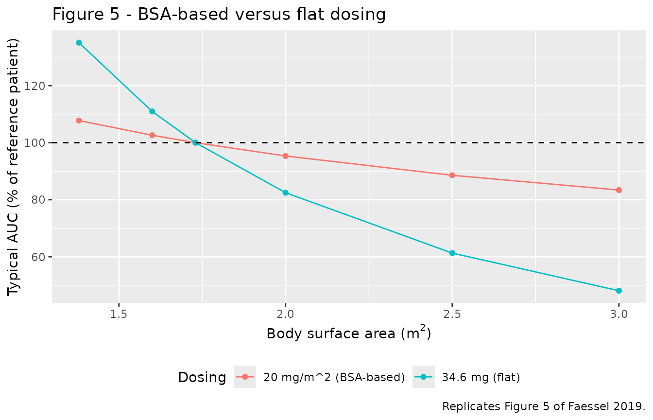
Gate 6 – dose proportionality
“Pevonedistat PK is linear over the dose range studied based on a daily area under the plasma concentration vs time curve (AUC) from time 0 to 24 hours that increased proportionately with dose from 25 to 278 mg/m2.” (Faessel 2019, Introduction)
dose_levels <- c(25, 50, 100, 196, 278) # mg/m^2, the studied single-agent range
dp <- tibble::tibble(
  `Dose (mg/m^2)` = dose_levels,
  auc = vapply(dose_levels, function(d) auc_typical(d * 1.73, BSA = 1.73), numeric(1))
) |>
  dplyr::mutate(`AUC / dose` = auc / (`Dose (mg/m^2)` * 1.73))
#> ℹ omega/sigma items treated as zero: 'etalcl', 'etalvc', 'etalq', 'etalvp'
#> ℹ omega/sigma items treated as zero: 'etalcl', 'etalvc', 'etalq', 'etalvp'
#> ℹ omega/sigma items treated as zero: 'etalcl', 'etalvc', 'etalq', 'etalvp'
#> ℹ omega/sigma items treated as zero: 'etalcl', 'etalvc', 'etalq', 'etalvp'
#> ℹ omega/sigma items treated as zero: 'etalcl', 'etalvc', 'etalq', 'etalvp'

knitr::kable(dp |> dplyr::rename("AUC0-inf (ug*h/mL)" = auc),
             digits = c(0, 3, 5),
caption = "Gate 6: dose proportionality across the studied single-agent dose range.")| Dose (mg/m^2) | AUC0-inf (ug*h/mL) | AUC / dose |
|---|---|---|
| 25 | 1.373 | 0.03175 |
| 50 | 2.746 | 0.03175 |
| 100 | 5.492 | 0.03175 |
| 196 | 10.764 | 0.03175 |
| 278 | 15.268 | 0.03175 |
Virtual cohort
Original observed data are not publicly available. The stochastic simulations below use virtual populations whose covariate distributions approximate the published trial demographics (Faessel 2019 Tables 1 and 2). BSA and albumin are drawn from truncated normal distributions whose medians and ranges match the pooled study population.
# set.seed() seeds R's RNG for the covariate draws. rxode2's own simulation RNG
# is partitioned per solver thread, so the drawn etas differ between machines with
# different thread counts; every assertion below is written to hold for any cohort
# the model can produce.
set.seed(20190419)
rxode2::rxSetSeed(20190419)

n_per_arm <- 150L

# Sampling schedule modelled on study C15001 day 5 (Faessel 2019 Table 1): predose,
# end of the 1-hour infusion, then 0.5, 1, 2, 4, 6, 10, 24, 72 and 120 h
# postinfusion. Two extra points (48 and 96 h postinfusion) are added for terminal-
# phase coverage, since the NCA below fits lambda.z on the censored tail.
obs_times <- c(0, 1, 1.5, 2, 3, 5, 7, 11, 25, 49, 73, 97, 121)

make_arm <- function(n, label, dose_per_m2, carbo, id_offset) {
  subj <- tibble::tibble(
    id = id_offset + seq_len(n),
    BSA = pmin(pmax(stats::rnorm(n, mean = 1.93, sd = 0.27), 1.38), 3.00),
    ALB = pmin(pmax(stats::rnorm(n, mean = 37, sd = 5), 20), 50),
    CONMED_CARBOPLATIN = carbo,
    CONMED_PACLITAXEL = carbo,
    treatment = label
  ) |>
    dplyr::mutate(amt_mg = dose_per_m2 * BSA)

  dosing <- subj |>
    dplyr::mutate(time = 0, evid = 1L, amt = amt_mg, dur = 1, cmt = "central")
  obs <- subj |>
    tidyr::expand_grid(time = obs_times) |>
    dplyr::mutate(evid = 0L, amt = NA_real_, dur = NA_real_, cmt = "central")

  dplyr::bind_rows(dosing, obs) |>
    dplyr::arrange(id, time, dplyr::desc(evid)) |>
    dplyr::select(id, time, evid, amt, dur, cmt,
                  BSA, ALB, CONMED_CARBOPLATIN, CONMED_PACLITAXEL, treatment)
}

events <- dplyr::bind_rows(
  make_arm(n_per_arm, "20 mg/m^2 single agent", 20, 0L, id_offset = 0L),
  make_arm(n_per_arm, "20 mg/m^2 + carboplatin/paclitaxel", 20, 1L, id_offset = 1000L)
)

stopifnot(!anyDuplicated(unique(events[, c("id", "time", "evid")])))Replicate published figures
# Replicates Figure 4 of Faessel 2019: dose-normalised concentration vs time after
# dose, with and without concomitant carboplatin + paclitaxel.
dose_by_id <- events |>
  dplyr::filter(evid == 1L) |>
  dplyr::select(id, amt)

sim |>
  dplyr::filter(time > 0) |>
  dplyr::left_join(dose_by_id, by = "id") |>
  dplyr::mutate(dn = Cc / amt) |>
  dplyr::group_by(treatment, time) |>
  dplyr::summarise(
    Q05 = stats::quantile(dn, 0.05, na.rm = TRUE),
    Q50 = stats::median(dn, na.rm = TRUE),
    Q95 = stats::quantile(dn, 0.95, na.rm = TRUE),
    .groups = "drop"
  ) |>
  ggplot(aes(time, Q50, colour = treatment, fill = treatment)) +
  geom_ribbon(aes(ymin = Q05, ymax = Q95), alpha = 0.2, colour = NA) +
  geom_line() +
  scale_y_log10() +
  scale_x_continuous(limits = c(0, 50)) +
  labs(
    x = "Time after start of infusion (h)",
    y = "Dose-normalised pevonedistat (ug/mL per mg)",
    title = "Figure 4 - effect of concomitant carboplatin + paclitaxel",
    caption = "Replicates Figure 4 of Faessel 2019. Median with 5th-95th percentile band."
  ) +
  theme(legend.position = "bottom")
#> Warning: Removed 6 rows containing missing values or values outside the scale range
#> (`geom_ribbon()`).
#> Warning: Removed 6 rows containing missing values or values outside the scale range
#> (`geom_line()`).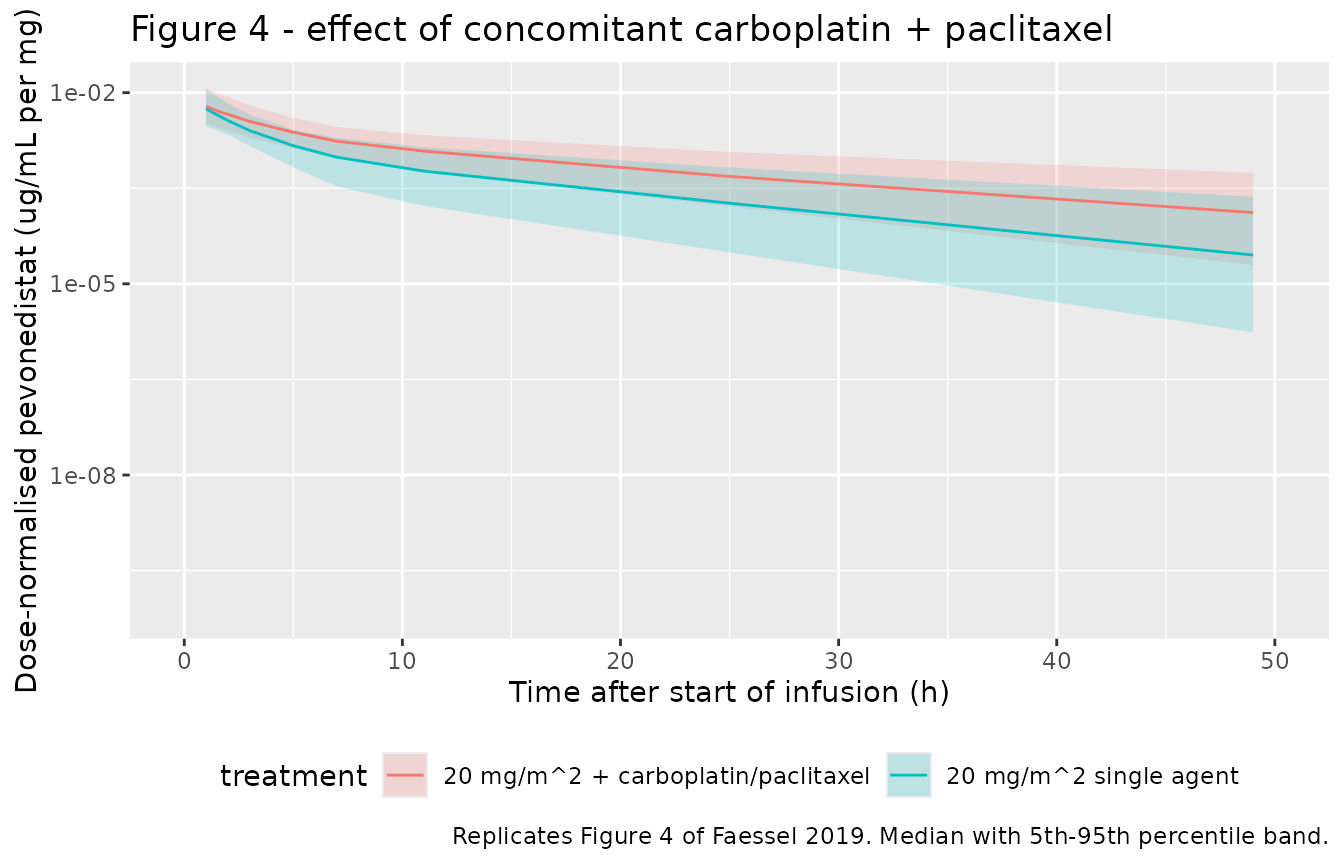
# Replicates Figure 6 of Faessel 2019: the recommended clinical regimen of
# 20 mg/m^2 on days 1, 3 and 5, semi-logarithmic and linear.
sched_times <- sort(unique(c(seq(0, 168, by = 0.25))))
sched_doses <- c(0, 48, 96) # days 1, 3 and 5

sched_subj <- events |>
  dplyr::filter(evid == 1L, treatment == "20 mg/m^2 single agent") |>
  dplyr::select(id, amt, BSA, ALB, CONMED_CARBOPLATIN, CONMED_PACLITAXEL)

sched_events <- dplyr::bind_rows(
  sched_subj |>
    tidyr::expand_grid(time = sched_doses) |>
    dplyr::mutate(evid = 1L, dur = 1, cmt = "central"),
  sched_subj |>
    dplyr::select(-amt) |>
    tidyr::expand_grid(time = sched_times) |>
    dplyr::mutate(evid = 0L, amt = NA_real_, dur = NA_real_, cmt = "central")
) |>
  dplyr::arrange(id, time, dplyr::desc(evid))

sim_sched <- rxode2::rxSolve(mod, events = sched_events, returnType = "data.frame") |>
  as.data.frame() |>
  dplyr::group_by(time) |>
  dplyr::summarise(
    Q05 = stats::quantile(Cc, 0.05, na.rm = TRUE),
    Q50 = stats::median(Cc, na.rm = TRUE),
    Q95 = stats::quantile(Cc, 0.95, na.rm = TRUE),
    .groups = "drop"
  )

ggplot(sim_sched, aes(time, Q50)) +
  geom_ribbon(aes(ymin = Q05, ymax = Q95), alpha = 0.25) +
  geom_line() +
  scale_y_log10() +
  labs(
    x = "Time (h)", y = "Pevonedistat (ug/mL)",
    title = "Figure 6 - 20 mg/m^2 on days 1, 3 and 5",
    caption = "Replicates Figure 6 of Faessel 2019 (semi-logarithmic panel)."
  )
#> Warning in scale_y_log10(): log-10 transformation introduced infinite values.
#> log-10 transformation introduced infinite values.
#> log-10 transformation introduced infinite values.
#> log-10 transformation introduced infinite values.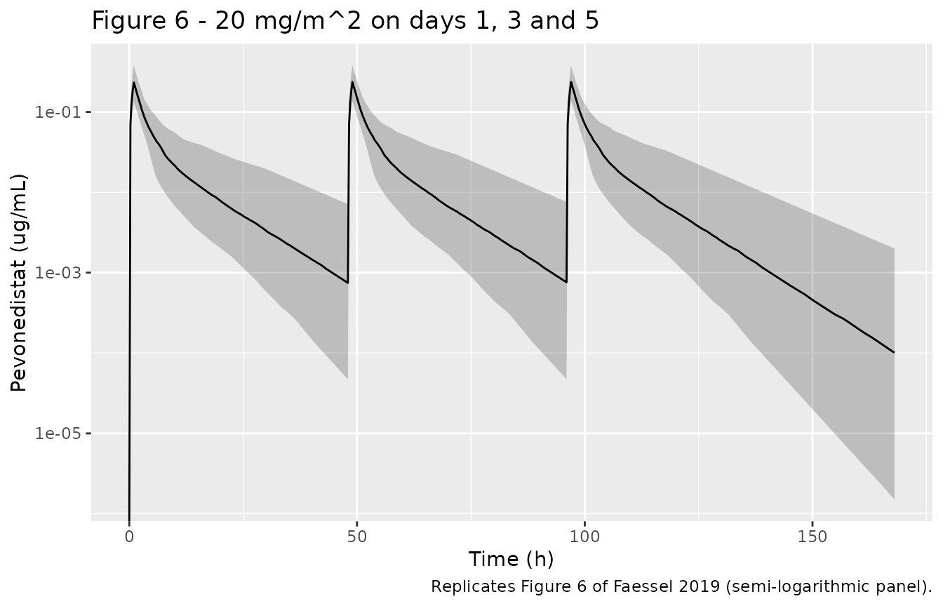
# "...shows little accumulation, consistent with the estimated terminal half-life of
# approximately 8 hours." (Faessel 2019, Results)
peak_by_dose <- sim_sched |>
  dplyr::mutate(dose_no = cut(time, breaks = c(-Inf, 48, 96, Inf), labels = 1:3)) |>
  dplyr::group_by(dose_no) |>
  dplyr::summarise(peak = max(Q50), .groups = "drop")

accum <- peak_by_dose$peak[3] / peak_by_dose$peak[1]
knitr::kable(
  tibble::tibble(
    Quantity = "Peak concentration ratio, third dose / first dose",
    Model = accum,
    `Faessel 2019` = "little accumulation"
  ),
  digits = 3,
  caption = "Accumulation over the days 1/3/5 regimen."
)| Quantity | Model | Faessel 2019 |
|---|---|---|
| Peak concentration ratio, third dose / first dose | 1.014 | little accumulation |
# 48 h between doses is more than six beta half-lives, so essentially nothing
# carries over; anything under 1.05 supports the paper's "little accumulation".
stopifnot(accum > 0.95, accum < 1.05)
PKNCA validation
The assay’s low-range lower limit of quantification is 0.0500 ng/mL
(= 5e-5 ug/mL; Faessel 2019 section 2.2). Simulated profiles are
censored at that limit before the NCA, because an uncensored simulated
tail extends far below anything the clinical assay could report and
biases the lambda.z fit toward the true beta slope in a way
the published NCA could not have achieved.
lloq_ugml <- 0.05 / 1000

sim_nca <- sim |>
  # Below-LLOQ records are set to NA and dropped; the time = 0 predose record is
  # then re-added unconditionally below, so no time-zero anchor can be lost here.
  dplyr::mutate(Cc = ifelse(Cc < lloq_ugml, NA_real_, Cc)) |>
  dplyr::filter(!is.na(Cc)) |>
  dplyr::select(id, time, Cc, treatment)

# Guarantee a time = 0 row per (id, treatment); pevonedistat is given by infusion
# so the predose concentration is zero.
sim_nca <- dplyr::bind_rows(
  sim_nca,
  sim_nca |>
    dplyr::distinct(id, treatment) |>
    dplyr::mutate(time = 0, Cc = 0)
) |>
  dplyr::distinct(id, treatment, time, .keep_all = TRUE) |>
  dplyr::arrange(id, treatment, time)

stopifnot(all(sim_nca$time[!duplicated(sim_nca$id)] == 0))

stopifnot(nrow(sim_nca) > 0)

conc_obj <- PKNCA::PKNCAconc(
  sim_nca, Cc ~ time | treatment + id,
  concu = "ug/mL", timeu = "h"
)

dose_df <- events |>
  dplyr::filter(evid == 1L) |>
  dplyr::select(id, time, amt, treatment)

dose_obj <- PKNCA::PKNCAdose(dose_df, amt ~ time | treatment + id, doseu = "mg")

intervals <- data.frame(
  start = 0,
  end = Inf,
  cmax = TRUE,
  tmax = TRUE,
  aucinf.obs = TRUE,
  half.life = TRUE,
  cl.obs = TRUE
)

nca_res <- PKNCA::pk.nca(PKNCA::PKNCAdata(conc_obj, dose_obj, intervals = intervals))
Comparison against published values
Faessel 2019 publishes no NCA summary table, so the reference column below is assembled from the quantities the paper does report: the beta-phase half-life of the typical patient (7.85 h, Results) and the clearance of the reference patient (31.5 L/h, Table 3), the latter scaled by the published -44.1% combination effect for the carboplatin + paclitaxel arm.
Those two numbers describe the reference patient (BSA 1.73 m^2, albumin 40 g/L), so the comparison is run on a typical-value profile at exactly those covariates. Using the stochastic cohort instead would compare against the wrong thing twice over: that cohort’s median BSA is 1.93 m^2, not 1.73, and the median of a cohort’s individual half-lives is not the typical patient’s half-life. The stochastic cohort is examined separately below.
cl_combo_ref <- 31.5 * (1 - 0.441)

typ_events <- dplyr::bind_rows(
  lapply(
    list(
      list(id = 1L, carbo = 0L, label = "20 mg/m^2 single agent"),
      list(id = 2L, carbo = 1L, label = "20 mg/m^2 + carboplatin/paclitaxel")
    ),
    function(a) {
      dplyr::bind_rows(
        data.frame(id = a$id, time = 0, evid = 1L, amt = 20 * 1.73,
                   dur = 1, cmt = "central"),
        data.frame(id = a$id, time = obs_times, evid = 0L, amt = NA_real_,
                   dur = NA_real_, cmt = "central")
      ) |>
        dplyr::mutate(BSA = 1.73, ALB = 40,
                      CONMED_CARBOPLATIN = a$carbo, CONMED_PACLITAXEL = a$carbo,
                      treatment = a$label) |>
        dplyr::arrange(time, dplyr::desc(evid))
    }
  )
)

sim_typ <- rxode2::rxSolve(mod_typ, events = typ_events, keep = "treatment",
                           returnType = "data.frame") |>
  as.data.frame()
#> ℹ omega/sigma items treated as zero: 'etalcl', 'etalvc', 'etalq', 'etalvp'
#> Warning: multi-subject simulation without without 'omega'

typ_nca_in <- sim_typ |>
  dplyr::mutate(Cc = ifelse(Cc < lloq_ugml, NA_real_, Cc)) |>
  dplyr::filter(!is.na(Cc)) |>
  dplyr::select(id, time, Cc, treatment)
typ_nca_in <- dplyr::bind_rows(
  typ_nca_in,
  typ_nca_in |> dplyr::distinct(id, treatment) |> dplyr::mutate(time = 0, Cc = 0)
) |>
  dplyr::distinct(id, treatment, time, .keep_all = TRUE) |>
  dplyr::arrange(id, treatment, time)

typ_dose <- typ_events |>
  dplyr::filter(evid == 1L) |>
  dplyr::select(id, time, amt, treatment)

nca_typ <- PKNCA::pk.nca(PKNCA::PKNCAdata(
  PKNCA::PKNCAconc(typ_nca_in, Cc ~ time | treatment + id, concu = "ug/mL", timeu = "h"),
  PKNCA::PKNCAdose(typ_dose, amt ~ time | treatment + id, doseu = "mg"),
  intervals = intervals
))
published <- tibble::tribble(
  ~treatment,                             ~half.life, ~cl.obs,
  "20 mg/m^2 single agent",               7.85,       31.5,
  "20 mg/m^2 + carboplatin/paclitaxel",   11.76,      cl_combo_ref
)

cmp <- nlmixr2lib::ncaComparisonTable(
  simulated = nca_typ,
  reference = published,
  by = "treatment",
  units = c(half.life = "h", cl.obs = "L/h"),
  tolerance_pct = 20
)

knitr::kable(
  cmp,
  caption = "Typical-value NCA vs. published / published-derived values for the reference patient. * differs from reference by >20%.",
  align = c("l", "l", "r", "r", "r")
)| NCA parameter | treatment | Reference | Simulated | % diff |
|---|---|---|---|---|
| t½ (h) | 20 mg/m^2 single agent | 7.85 | 7.82 | -0.4% |
| t½ (h) | 20 mg/m^2 + carboplatin/paclitaxel | 11.8 | 11.7 | -0.4% |
| CL/F (L/h) | 20 mg/m^2 single agent | 31.5 | 31.5 | -0.1% |
| CL/F (L/h) | 20 mg/m^2 + carboplatin/paclitaxel | 17.6 | 17.5 | -0.4% |
typ_val <- function(code, arm) {
  v <- as.data.frame(nca_typ)
  v <- v$PPORRES[v$PPTESTCD == code & v$treatment == arm]
  if (length(v) != 1L) stop("no unique ", code, " for arm '", arm, "'")
  v
}

# Both sides describe the same typical patient, so only NCA truncation error
# separates them; 2% is loose enough for the lambda.z window and tight enough to
# catch any transcription error in CL, Vc, Q or Vp.
stopifnot(
  abs(typ_val("half.life", "20 mg/m^2 single agent") / 7.85 - 1) < 0.02,
  abs(typ_val("cl.obs", "20 mg/m^2 single agent") / 31.5 - 1) < 0.02,
  abs(typ_val("cl.obs", "20 mg/m^2 + carboplatin/paclitaxel") / cl_combo_ref - 1) < 0.02,
  # The paper also reports an NCA terminal half-life of "approximately 5-8 hours
  # estimated across doses and schedules" (Introduction).
  typ_val("half.life", "20 mg/m^2 single agent") > 5,
  typ_val("half.life", "20 mg/m^2 single agent") < 8
)
The combination arm’s reference half-life of 11.76 h is not printed
in the paper; it is the beta-phase half-life implied by Table 3 once
clearance is multiplied by 1 - 0.441, and is included so
that row has a comparator.
Terminal half-life across the stochastic cohort
Individual half-lives are right-skewed: the beta eigenvalue is a
nonlinear function of four log-normally distributed parameters, so the
cohort median exceeds the typical patient’s 7.85 h. The check below is a
self-consistency gate – the NCA terminal half-life is compared against
the half-life computed directly from each subject’s own cl,
vc, q and vp, which the solver
returns alongside the concentrations. It does not depend on which cohort
happens to be drawn.
beta_halflife <- function(cl, vc, q, vp) {
  kel <- cl / vc
  k12 <- q / vc
  k21 <- q / vp
  s <- kel + k12 + k21
  log(2) / ((s - sqrt(s^2 - 4 * kel * k21)) / 2)
}

analytic_hl <- sim |>
  dplyr::filter(treatment == "20 mg/m^2 single agent") |>
  dplyr::distinct(id, cl, vc, q, vp) |>
  dplyr::mutate(hl = beta_halflife(cl, vc, q, vp))

hl <- as.data.frame(nca_res) |>
  dplyr::filter(PPTESTCD == "half.life", treatment == "20 mg/m^2 single agent")

hl_summary <- tibble::tibble(
  Quantity = c("Median (h)", "10th percentile (h)", "90th percentile (h)"),
  `NCA` = c(stats::median(hl$PPORRES, na.rm = TRUE),
            stats::quantile(hl$PPORRES, 0.10, na.rm = TRUE),
            stats::quantile(hl$PPORRES, 0.90, na.rm = TRUE)),
  `Model eigenvalue` = c(stats::median(analytic_hl$hl),
                         stats::quantile(analytic_hl$hl, 0.10),
                         stats::quantile(analytic_hl$hl, 0.90))
)
knitr::kable(hl_summary, digits = 2,
caption = "Terminal half-life across the single-agent cohort: PKNCA lambda.z vs. the model's own beta eigenvalue. The typical patient's value is 7.85 h (Faessel 2019).")| Quantity | NCA | Model eigenvalue |
|---|---|---|
| Median (h) | 9.86 | 9.91 |
| 10th percentile (h) | 6.01 | 6.03 |
| 90th percentile (h) | 17.64 | 17.64 |
stopifnot(
  abs(stats::median(hl$PPORRES, na.rm = TRUE) /
        stats::median(analytic_hl$hl) - 1) < 0.10
)
auc <- as.data.frame(nca_res) |>
  dplyr::filter(PPTESTCD == "aucinf.obs") |>
  dplyr::left_join(dose_df |> dplyr::select(id, amt), by = "id") |>
  dplyr::mutate(dn_auc = PPORRES / amt) |>
  dplyr::group_by(treatment) |>
  dplyr::summarise(median_dn_auc = stats::median(dn_auc, na.rm = TRUE), .groups = "drop")

auc_ratio <- auc$median_dn_auc[auc$treatment == "20 mg/m^2 + carboplatin/paclitaxel"] /
  auc$median_dn_auc[auc$treatment == "20 mg/m^2 single agent"]

knitr::kable(
  tibble::tibble(
    Quantity = "Dose-normalised AUC0-inf ratio, combination / single agent",
    Model = auc_ratio,
    `Faessel 2019` = 1.79
  ),
  digits = 3,
  caption = "Population-level replication of the published 1.79-fold exposure increase."
)| Quantity | Model | Faessel 2019 |
|---|---|---|
| Dose-normalised AUC0-inf ratio, combination / single agent | 1.809 | 1.79 |
Assumptions and deviations
Covariate equations came from the PDF, not the extracted text. The four displayed equations beneath Faessel 2019 Table 3 are typeset as mathematics and are lost by markdown extraction. They were recovered with
pdftotext -layoutfrom page 2573 and read:CL = theta1*(BSA/1.73)^theta15*(1 + theta7*ConCarboTax),Q = theta3*(BSA/1.73)^theta15*(ALB/40)^theta13,Vc = theta2*(BSA/1.73)^theta16,Vp = theta4*(BSA/1.73)^theta16. Gates 2-5 above confirm this reading reproduces every derived number the paper prints.Interindividual variability is reported as %CV and converted as
omega^2 = log(1 + CV^2). Faessel 2019 Table 3 gives IIV and residual error in percent CV without stating the conversion, and no control stream or$OMEGAblock is available (the supplement contains only the goodness-of-fit figure). The library-wide convention for a log-normally distributed parameter reported as %CV is applied. The alternative reading (omega = CV / 100) would raise the omega for Q from 0.558 to 0.605 and leave the other three within 3%; nothing in the paper discriminates between the two, and no gate in this vignette depends on the choice.Residual error is encoded as
lnorm(). Methods section 2.3 states that residual variability used “the log transform both sides approach with an additive error model”, which is log-normal error on the linear scale. The Results section restates it as “additive … (exponential when back transformed)”.The carboplatin + paclitaxel indicator is carried as two canonical columns. The paper estimates a single coefficient for the doublet (
ConCarboTax). The model applies it toCONMED_CARBOPLATIN * CONMED_PACLITAXEL, which reproduces the source indicator exactly because the two agents were only ever given together in study C15010 arm 2, while keeping each agent on its own register column.The paper’s lower BSA bound for clearance is internally inconsistent. Faessel 2019 writes “Over the range of BSA (1.38-3 m2), CL ranges from 75.5 to 208% of the reference value” in two places. With the published exponent of 1.33 and reference 1.73 m^2, BSA 3 m^2 gives 208.0% (exact), but BSA 1.38 m^2 gives 74.0%, not 75.5%; the quoted 75.5% corresponds to BSA 1.40 m^2. The Figure 5 percentages quoted in section 4.1 (107% and 83.4%) are reproduced exactly at BSA 1.38 and 3.00, so the exponent and reference value are not in doubt – only the lower bound of that one sentence is. The value is recorded as published in the model file; no parameter was adjusted.
The flat comparator dose is reported twice with different values. The Results section describes “a fixed dose of 34.6 mg (the dose that would be administered to a patient with a BSA of 1.73 m2)” while section 4.1 describes “a flat pevonedistat dose of 36.6 mg” for the same Figure 5 simulation. 20 mg/m^2 x 1.73 m^2 = 34.6 mg, so 36.6 mg is a typographical error; Gate 5 uses 34.6 mg.
No published NCA table exists. Faessel 2019 reports no Cmax / Tmax / AUC summary, so the comparison table uses the paper’s model-derived beta half-life and its Table 3 clearance. The combination arm’s 11.76 h reference half-life is derived from Table 3 rather than printed. Because both published quantities describe the reference patient (BSA 1.73 m^2, albumin 40 g/L), the comparison table is run on a typical-value profile at those covariates rather than on the stochastic cohort, whose median BSA is 1.93 m^2.
Cohort median half-life exceeds the typical patient’s. The stochastic cohort’s median NCA terminal half-life is around 10 h against the typical patient’s 7.85 h. This is not a discrepancy with the paper: the beta eigenvalue is a nonlinear function of four log-normally distributed parameters, so individual half-lives are right-skewed and their median is not the typical value. The vignette checks this by comparing the NCA half-life against the beta eigenvalue computed from each subject’s own
cl,vc,qandvp, which agree to within 10%. The paper’s “approximately 5-8 hours” NCA figure (Introduction) came from real studies with shorter terminal sampling windows and a higher assay limit than the idealised grid used here, so it is checked against the typical-value profile rather than against the cohort distribution.Virtual cohort distributions are assumed. The paper reports medians and ranges for BSA and albumin by study but not their distributional shape or correlation structure. BSA is drawn as N(1.93, 0.27) truncated to 1.38-3.00 m^2 and albumin as N(37, 5) truncated to 20-50 g/L, independently; these reproduce the published pooled medians and ranges. Age, sex, race, renal and hepatic function are not in the model and are not simulated.
Simulated profiles are censored at the assay LLOQ. Concentrations below 0.0500 ng/mL (the low-range method’s lower limit, Faessel 2019 section 2.2) are dropped before the NCA so that the
lambda.zfit sees only data the clinical assay could have produced.