Vancomycin (Takada 2025)
Source:vignettes/articles/Takada_2025_vancomycin.Rmd
Takada_2025_vancomycin.RmdModel and source
- Citation: Takada K, Samura M, Igarashi Y, Suzuki A, Ishigo T, Fujii S, Ibe Y, Yoshida H, Tanaka H, Ebihara F, Maruyama T, Hamada Y, Komatsu T, Tomizawa A, Takuma A, Chiba H, Yagi Y, Nishi Y, Enoki Y, Taguchi K, Tanikawa K, Kunishima H, Matsumoto K. Development and validation of a population pharmacokinetic model of vancomycin for patients of advanced age. J Pharm Health Care Sci. 2025;11(1):18. doi:10.1186/s40780-025-00423-8.
- Description: Two-compartment IV population PK model for vancomycin in Japanese patients of advanced age (aged 75 years and older, body mass index below 25 kg/m^2) receiving therapeutic drug monitoring (Takada 2025). Clearance scales as a power function of Cockcroft-Gault creatinine clearance (exponent 0.63, reference 3.09 L/h = 51.5 mL/min) and of serum albumin (exponent 0.22, reference 2.3 g/dL); the albumin term is the novelty of this analysis, added because creatinine-based renal-function estimates underestimate clearance in low-muscle-mass patients of advanced age. Intercompartmental clearance and both volumes are covariate-free. Between-subject variability is on clearance only; the residual-error magnitudes were not reported by the source and are encoded as zero.
- Article: https://doi.org/10.1186/s40780-025-00423-8
- Supplement (Additional Files 1-10, Springer ESM): https://static-content.springer.com/esm/art%3A10.1186%2Fs40780-025-00423-8/MediaObjects/40780_2025_423_MOESM1_ESM.docx
(files
MOESM1throughMOESM10)
Note on supplement numbering: the paper’s “Additional File
N” labels do not line up with the MOESM file
indices on the publisher’s server. The two load-bearing files here are
the renal-function equations (the paper’s Additional File 2: Table 2,
served as MOESM4) and the clearance nomogram (Additional
File 6: Table 5, served as MOESM7). Citations below give
both the paper’s label and the file index so either route reaches the
right table.
Takada 2025 develops a two-compartment intravenous population PK model for vancomycin in Japanese inpatients aged 75 years and older with a body mass index below 25 kg/m^2. The analysis is motivated by a specific clinical failure mode: creatinine-based renal-function equations systematically underestimate clearance in patients of advanced age with low muscle mass, so a model that carries only creatinine clearance mis-predicts vancomycin clearance in exactly the patients most at risk. The paper’s contribution is the addition of serum albumin as a second covariate on clearance – albumin correlates with muscle mass in this age group – which lowered the objective function by 5.11 points over the creatinine-clearance-only model (Table 2, model 4 versus model 3) and gave the lowest mean absolute and mean squared prediction error of any tested model in the subgroup with serum creatinine below 0.6 mg/dL.
Population
The model was fit to 417 vancomycin concentrations (65 peaks, 352 troughs) from 159 patients treated at Yokohama General Hospital between August 2016 and September 2024 (Takada 2025 Table 1). Median age was 84 years (range 75-99), with 49.7% aged 85 or older; 42.1% were female. The cohort was small and frail: median body weight 47 kg (range 26-70), median body mass index 18.6 kg/m^2 (range 11.0-24.8, with 48.4% below 18.5), and median serum albumin 2.3 g/dL (range 1.2-4.2, with 90.6% below 3.0 g/dL). Median Cockcroft-Gault creatinine clearance was 51.5 mL/min (range 9.7-121.2) and median serum creatinine 0.64 mg/dL (range 0.22-3.00), with 42.1% below 0.60 mg/dL. Daily maintenance doses were chosen by the treating physician, median 1500 mg/day (range 250-3000). Patients on dialysis, patients treated for fewer than three days, and patients with no vancomycin sample were excluded.
A separate 133-patient multicentre cohort (eight hospitals, September 2020 to December 2023) was used only for external validation of predictive performance and contributed nothing to the parameter estimates reproduced here.
The same information is available programmatically via the model’s
population metadata
(readModelDb("Takada_2025_vancomycin")()$population).
Source trace
The per-parameter origin is recorded as an in-file comment next to
each ini() entry in
inst/modeldb/specificDrugs/Takada_2025_vancomycin.R. The
table below collects them in one place for review.
| Equation / parameter | Value | Source location |
|---|---|---|
lcl (CL at reference covariates) |
1.96 L/h | Table 3, theta1 (SE 0.06, CV 3.11%, 95% CI 1.84-2.08) |
e_crcl_cl (exponent on CLcr) |
0.63 | Table 3, theta2 (SE 0.06, CV 9.72%, 95% CI 0.51-0.76) |
e_alb_cl (exponent on Alb) |
0.22 | Table 3, theta3 (SE 0.09, CV 41.75%, 95% CI 0.03-0.40) |
lq (intercompartmental clearance) |
4.86 L/h | Table 3, theta4 (SE 0.91, CV 18.63%, 95% CI 3.08-6.64); Abstract agrees. See Errata for the conflicting 3.24 in the Results narrative |
lvc (central volume) |
31.78 L | Table 3, theta5 (SE 3.86, CV 12.16%, 95% CI 24.19-39.38) |
lvp (peripheral volume) |
53.64 L | Table 3, theta6 (SE 4.22, CV 7.86%, 95% CI 45.36-61.93) |
etalcl (IIV variance on CL) |
0.11 | Table 3 footnote: “eta … normally distributed with mean 0 and variance omega^2, etaCL = 0.11” |
propSd, addSd
|
0 (fixed) | Not reported. Additional File 1: Table 1 (file MOESM3) lists the three candidate residual models evaluated but no estimate is published anywhere. See Errata |
| CL covariate equation | 1.96 * (CLcr/3.09)^0.63 * (Alb/2.3)^0.22 * exp(etaCL) |
Table 3 header row and Results, “Development of a population pharmacokinetic model” |
| Reference CLcr = 3.09 L/h | 51.5 mL/min | Table 1 modeling-cohort median estimated creatinine clearance |
| Reference Alb = 2.3 g/dL | 23 g/L | Table 1 modeling-cohort median serum albumin |
| CLcr estimating equation |
([140 - age] * BW) / (SCr * 72), female
* 0.85
|
Additional File 2: Table 2 (file MOESM4), Equations 1-2 |
| Two-compartment structure | n/a | Methods (“one- or two-compartment models of the first-order elimination were fitted”); Results, “A two-compartment model was optimal for VCM” |
| Published CL nomogram | 70-cell grid | Additional File 6: Table 5 (file MOESM7) |
| Published dose nomogram | 70-cell grid | Table 4 |
| Published safety nomogram | 70-cell risk grid | Additional File 10: Table 8 (file MOESM10); legend: low risk below 10%, moderate 10 to below 25%, high 25% or above |
| MIC distribution used for target attainment | 0.25: 0.1%, 0.5: 11.6%, 1.0: 79.3%, 2.0: 9.0% (ug/mL) | Methods, Monte Carlo section, citing the 2019 Japanese MRSA guidelines |
mod <- readModelDb("Takada_2025_vancomycin")
ui <- rxode2::rxode(mod)
#> ℹ parameter labels from comments will be replaced by 'label()'
ui$iniDf |>
  dplyr::filter(!is.na(ntheta)) |>
  dplyr::select(name, est, fix, label) |>
  dplyr::rename(
    "Parameter" = name, "Estimate" = est, "Fixed" = fix, "Label" = label
  ) |>
knitr::kable(caption = "Packaged `ini()` values (log-scale entries shown as stored).")| Parameter | Estimate | Fixed | Label |
|---|---|---|---|
| lcl | 0.6729445 | FALSE | Clearance at CLcr=3.09 L/h and Alb=2.3 g/dL (L/h) |
| lq | 1.5810384 | FALSE | Intercompartmental clearance (L/h) |
| lvc | 3.4588372 | FALSE | Central volume of distribution (L) |
| lvp | 3.9822951 | FALSE | Peripheral volume of distribution (L) |
| e_crcl_cl | 0.6300000 | FALSE | Power exponent on (CLcr/3.09 L/h) for CL (unitless) |
| e_alb_cl | 0.2200000 | FALSE | Power exponent on (Alb/2.3 g/dL) for CL (unitless) |
| propSd | 0.0000000 | TRUE | Proportional residual SD (fraction; 0 – not reported in the source) |
| addSd | 0.0000000 | TRUE | Additive residual SD (ug/mL; 0 – not reported in the source) |
Check 1 – the published clearance nomogram (Additional File 6: Table 5, file MOESM7)
Takada 2025 prints a 70-cell grid of typical clearance over
creatinine clearance 1.2-5.1 L/h (20-85 mL/min) and serum albumin
1.5-3.5 g/dL. That grid is a direct, closed-form test of the covariate
equation: if the packaged parameters and the unit conversions in
model() are right, the equation must reproduce every
published cell.
There is one wrinkle, which is a property of the paper and not of
this implementation. The paper’s own nomogram substitutes the
constant 0.11 into the exp(etaCL) term, treating
the between-subject variance as a fixed multiplier of
exp(0.11) = 1.1163. That is confirmed by the Discussion,
which quotes CL = 2.73 and 3.29 L/h at CLcr 5.1 L/h for albumin 1.5 and
3.5 g/dL – values that are only recovered with the extra factor. The
packaged model treats etaCL correctly, as a mean-zero
random effect with variance 0.11, so its typical-value clearance is
exactly exp(0.11) = 11.6% below every printed cell. Both
readings are shown below.
crcl_grid <- c(1.2, 1.5, 1.8, 2.1, 2.4, 2.7, 3.0, 3.3, 3.6, 3.9, 4.2, 4.5, 4.8, 5.1)
alb_grid  <- c(1.5, 2.0, 2.5, 3.0, 3.5)

# Takada 2025 Additional File 6: Table 5 (file MOESM7), transcribed as printed.
published_cl <- matrix(
  c(1.09, 1.25, 1.41, 1.55, 1.69, 1.82, 1.95, 2.07, 2.19, 2.30, 2.41, 2.52, 2.62, 2.73,
    1.16, 1.34, 1.50, 1.65, 1.80, 1.94, 2.07, 2.20, 2.33, 2.45, 2.57, 2.68, 2.80, 2.91,
    1.22, 1.40, 1.58, 1.74, 1.89, 2.04, 2.18, 2.32, 2.45, 2.57, 2.70, 2.82, 2.94, 3.05,
    1.27, 1.46, 1.64, 1.81, 1.97, 2.12, 2.27, 2.41, 2.55, 2.68, 2.81, 2.93, 3.06, 3.18,
    1.31, 1.51, 1.70, 1.87, 2.04, 2.20, 2.35, 2.49, 2.64, 2.77, 2.91, 3.04, 3.16, 3.29),
  nrow = length(alb_grid), byrow = TRUE,
  dimnames = list(paste0("Alb ", alb_grid), paste0("CLcr ", crcl_grid))
)

cl_equation <- function(crcl, alb, eta = 0) {
  1.96 * (crcl / 3.09)^0.63 * (alb / 2.3)^0.22 * exp(eta)
}

recomputed_paper <- outer(alb_grid, crcl_grid, function(a, c) cl_equation(c, a, eta = 0.11))
recomputed_model <- outer(alb_grid, crcl_grid, function(a, c) cl_equation(c, a, eta = 0))

max_dev_paper <- max(abs(round(recomputed_paper, 2) - published_cl))
ratio <- published_cl / recomputed_model
rel_dev <- abs(ratio / exp(0.11) - 1)

stopifnot(
  # Every published cell is reproduced to within one unit in the last printed
  # decimal place when the paper's exp(0.11) convention is applied. (The
  # epsilon absorbs binary floating-point representation of 0.01, not any
  # real deviation.)
  max_dev_paper <= 0.01 + 1e-9,
  # ... and the offset from the packaged (eta = 0) typical value is exactly
  # exp(0.11) in all 70 cells, to within the granularity of the published
  # two-decimal rounding. A signature, not scatter: real parameter error would
  # vary systematically across the grid rather than sitting on a constant.
  all(rel_dev < 0.015),
  length(published_cl) == 70L
)

cat(sprintf(
  "All %d published cells reproduced; max absolute deviation %.3f L/h.\n",
  length(published_cl), max_dev_paper
))
#> All 70 published cells reproduced; max absolute deviation 0.010 L/h.
cat(sprintf(
  "published / packaged-typical ratio: %.4f to %.4f (exp(0.11) = %.4f);\n  max relative deviation from exp(0.11): %.2f%%.\n",
  min(ratio), max(ratio), exp(0.11), 100 * max(rel_dev)
))
#> published / packaged-typical ratio: 1.1047 to 1.1166 (exp(0.11) = 1.1163);
#>   max relative deviation from exp(0.11): 1.04%.
The Discussion’s two quoted values are recovered exactly:
tibble::tibble(
  `Quantity` = c("CL at CLcr 5.1 L/h, Alb 1.5 g/dL", "CL at CLcr 5.1 L/h, Alb 3.5 g/dL"),
  `Takada 2025 Discussion (L/h)` = c(2.73, 3.29),
  `Recomputed with exp(0.11) (L/h)` = round(c(cl_equation(5.1, 1.5, 0.11), cl_equation(5.1, 3.5, 0.11)), 2),
  `Packaged typical value (L/h)` = round(c(cl_equation(5.1, 1.5), cl_equation(5.1, 3.5)), 2)
) |>
knitr::kable(caption = "Takada 2025 Discussion cross-check of the clearance equation.")| Quantity | Takada 2025 Discussion (L/h) | Recomputed with exp(0.11) (L/h) | Packaged typical value (L/h) |
|---|---|---|---|
| CL at CLcr 5.1 L/h, Alb 1.5 g/dL | 2.73 | 2.73 | 2.45 |
| CL at CLcr 5.1 L/h, Alb 3.5 g/dL | 3.29 | 3.29 | 2.95 |
Virtual cohort
Original observed data are not publicly available. The simulations below use a virtual population whose demographics approximate the published modeling-cohort characteristics (Takada 2025 Table 1). Age, sex, body weight, serum creatinine, and serum albumin are sampled from truncated distributions matched to the published medians and ranges; creatinine clearance is then computed with the paper’s own Cockcroft-Gault equation (Additional File 2: Table 2, file MOESM4) rather than sampled directly, so the covariate pipeline is exercised end to end.
set.seed(20250307)

n_subj <- 159L  # matches the Takada 2025 modeling cohort

# Sample from a log-normal truncated to the published range, calibrated so the
# median equals the published median.
rtrunc_lnorm <- function(n, med, lo, hi, cv) {
  out <- numeric(0)
  while (length(out) < n) {
    draw <- stats::rlnorm(2 * n, meanlog = log(med), sdlog = sqrt(log(cv^2 + 1)))
    out <- c(out, draw[draw >= lo & draw <= hi])
  }
  out[seq_len(n)]
}

draw_subjects <- function(n) {
  tibble::tibble(
    AGE     = round(rtrunc_lnorm(n, med = 84,   lo = 75,   hi = 99,   cv = 0.07)),
    SEXF    = stats::rbinom(n, 1L, 0.421),
    WT      = round(rtrunc_lnorm(n, med = 47,   lo = 26,   hi = 70,   cv = 0.20), 1),
    CREAT   = round(rtrunc_lnorm(n, med = 0.64, lo = 0.22, hi = 3.00, cv = 0.55), 2),
    ALB_gdL = round(rtrunc_lnorm(n, med = 2.3,  lo = 1.2,  hi = 4.2,  cv = 0.22), 1)
  ) |>
    dplyr::mutate(
      # Takada 2025 Additional File 2: Table 2 (file MOESM4), Equations 1-2.
      CRCL = ((140 - AGE) * WT) / (CREAT * 72) * ifelse(SEXF == 1L, 0.85, 1),
      # Canonical ALB is SI g/L; the paper reports g/dL.
      ALB  = ALB_gdL * 10
    )
}

# Demographics are sampled independently, so a few draws combine into a
# creatinine clearance outside the observed range. Reject those rather than
# extrapolate the covariate model past the data it was fit to (Takada 2025
# Table 1 CLcr range 9.7-121.2 mL/min; the Limitations note that even the
# published extremes are sparsely populated).
cohort <- draw_subjects(8L * n_subj) |>
  dplyr::filter(CRCL >= 9.7, CRCL <= 121.2) |>
  dplyr::slice_head(n = n_subj) |>
  dplyr::mutate(id = seq_len(n_subj))
stopifnot(nrow(cohort) == n_subj)

# The cohort is only credible if the DERIVED creatinine clearance lands on the
# published distribution, so check it rather than assume it.
cohort_check <- tibble::tribble(
  ~Characteristic,                  ~`Takada 2025 Table 1`,     ~Simulated,
  "Age (years), median [range]",    "84 [75-99]",               sprintf("%.0f [%.0f-%.0f]", median(cohort$AGE), min(cohort$AGE), max(cohort$AGE)),
  "Female (%)",                     "42.1",                     sprintf("%.1f", 100 * mean(cohort$SEXF)),
  "Body weight (kg), median [range]", "47 [26-70]",             sprintf("%.0f [%.0f-%.0f]", median(cohort$WT), min(cohort$WT), max(cohort$WT)),
  "Serum creatinine (mg/dL), median [range]", "0.64 [0.22-3.00]", sprintf("%.2f [%.2f-%.2f]", median(cohort$CREAT), min(cohort$CREAT), max(cohort$CREAT)),
  "Serum albumin (g/dL), median [range]", "2.3 [1.2-4.2]",      sprintf("%.1f [%.1f-%.1f]", median(cohort$ALB_gdL), min(cohort$ALB_gdL), max(cohort$ALB_gdL)),
  "CLcr (mL/min), median [range]",  "51.5 [9.7-121.2]",         sprintf("%.1f [%.1f-%.1f]", median(cohort$CRCL), min(cohort$CRCL), max(cohort$CRCL))
)

knitr::kable(
  cohort_check,
  caption = "Virtual cohort versus the Takada 2025 modeling-cohort demographics. CLcr is derived from the sampled demographics via the paper's Cockcroft-Gault equation, not sampled."
)| Characteristic | Takada 2025 Table 1 | Simulated |
|---|---|---|
| Age (years), median [range] | 84 [75-99] | 85 [75-98] |
| Female (%) | 42.1 | 40.3 |
| Body weight (kg), median [range] | 47 [26-70] | 47 [28-70] |
| Serum creatinine (mg/dL), median [range] | 0.64 [0.22-3.00] | 0.65 [0.25-2.38] |
| Serum albumin (g/dL), median [range] | 2.3 [1.2-4.2] | 2.3 [1.5-4.1] |
| CLcr (mL/min), median [range] | 51.5 [9.7-121.2] | 51.6 [11.0-115.7] |
Simulation
Vancomycin is given as an intermittent intravenous infusion. Takada
2025 does not state the infusion duration, so a one-hour infusion is
assumed; steady-state exposure (AUCss), which is what the
paper’s targets and nomograms are built on, does not depend on that
choice. Three regimens spanning the published dose range are simulated
at steady state (ss = 1, ii = 12): 500, 750,
and 1000 mg every 12 hours, i.e. 1000, 1500 (the cohort median), and
2000 mg/day.
tau <- 12  # dosing interval (h)
obs_times <- seq(0, 24, by = 0.25)

make_arm <- function(cohort, dose_mg, label, id_offset) {
  covs <- cohort |>
    dplyr::mutate(id = id + id_offset, regimen = label) |>
    dplyr::select(id, regimen, CRCL, ALB)

  doses <- covs |>
    dplyr::mutate(
      time = 0, amt = dose_mg, rate = dose_mg / 1,  # 1-hour infusion
      evid = 1L, cmt = "central", ii = tau, ss = 1L, addl = 1L
    )
  obs <- covs |>
    tidyr::crossing(time = obs_times) |>
    dplyr::mutate(
      amt = NA_real_, rate = NA_real_, evid = 0L,
      cmt = "central",  # the ODE state, never the observable `Cc`
      ii = 0, ss = 0L, addl = 0L
    )
  dplyr::bind_rows(doses, obs) |> dplyr::arrange(id, time, dplyr::desc(evid))
}

events <- dplyr::bind_rows(
  make_arm(cohort,  500, "500 mg q12h",  id_offset =   0L),
  make_arm(cohort,  750, "750 mg q12h",  id_offset = 200L),
  make_arm(cohort, 1000, "1000 mg q12h", id_offset = 400L)
)
# Check the event table directly: wrapping this in `unique()` first would strip
# the very duplicates being tested for, making the assertion unfalsifiable.
stopifnot(!anyDuplicated(events[, c("id", "time", "evid")]))

# steady-state searches for long-half-life subjects exceed the default step budget
sim <- rxode2::rxSolve(mod, events = events, keep = c("regimen", "CRCL", "ALB"),
                       maxsteps = 1e6) |>
  as.data.frame()
#> ℹ parameter labels from comments will be replaced by 'label()'
stopifnot(nrow(sim) > 0L, !all(is.na(sim$Cc)))
Figure 1 – steady-state concentration-time profile
Takada 2025 Figure 1 is a visual predictive check of vancomycin concentration against time after dosing, with the 5th, 50th, and 95th percentiles of the prediction overlaid on the observations. The observed concentrations are not available, so the panel below shows the simulated percentile bands alone. The bands reflect between-subject variability in clearance (variance 0.11) and in the sampled covariates only; because Takada 2025 publishes no residual-error estimate, the packaged model carries none, so these bands are narrower than the paper’s.
# rxSolve returns observation rows only, and carries no `evid` column.
sim |>
  dplyr::group_by(regimen, time) |>
  dplyr::summarise(
    Q05 = stats::quantile(Cc, 0.05, na.rm = TRUE),
    Q50 = stats::quantile(Cc, 0.50, na.rm = TRUE),
    Q95 = stats::quantile(Cc, 0.95, na.rm = TRUE),
    .groups = "drop"
  ) |>
  ggplot(aes(time, Q50)) +
  geom_ribbon(aes(ymin = Q05, ymax = Q95), alpha = 0.25) +
  geom_line() +
  facet_wrap(~regimen) +
  labs(
    x = "Time after dose (h)", y = "Vancomycin concentration (ug/mL)",
    title = "Steady-state vancomycin profiles",
    caption = "Structure of Figure 1 of Takada 2025 (5th / 50th / 95th percentiles); observed data not available."
  ) +
  theme_bw()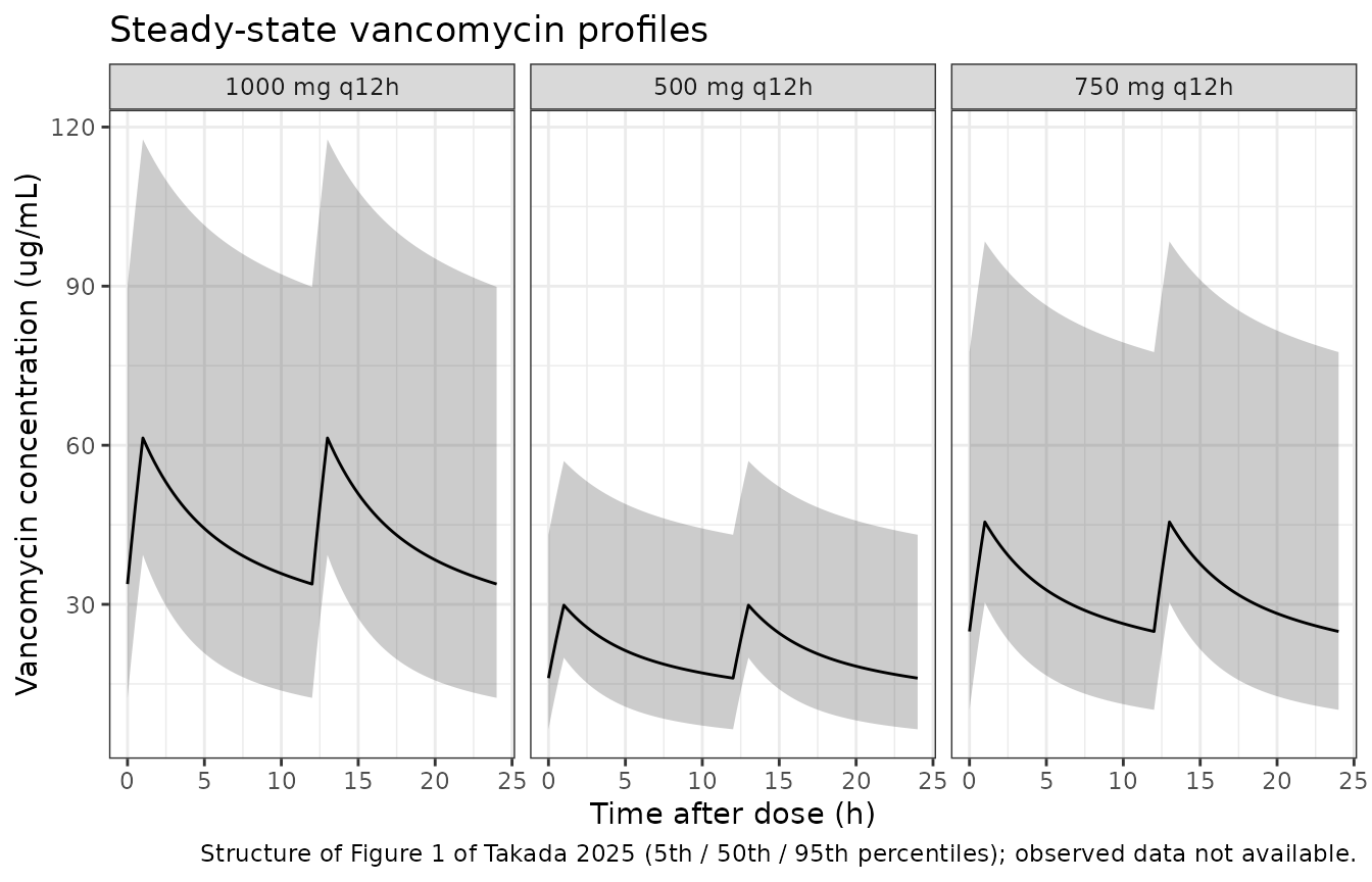
PKNCA validation
Non-compartmental analysis is run over the steady-state dosing
interval (0 to 12 h), which under ss = 1 is a genuine
steady-state interval.
sim_nca <- sim |>
  dplyr::filter(time <= tau) |>
  dplyr::filter(!is.na(Cc)) |>
  dplyr::select(id, time, Cc, regimen)

# Time-zero records are produced by the observation grid; assert rather than assume.
stopifnot(all(sim_nca |> dplyr::group_by(id) |> dplyr::summarise(z = any(time == 0)) |> dplyr::pull(z)))

conc_obj <- PKNCA::PKNCAconc(
  as.data.frame(sim_nca), Cc ~ time | regimen + id,
  concu = "ug/mL", timeu = "h"
)

# One dose row per subject anchors the interval so `cl.last` is Dose_tau / AUC_tau.
dose_df <- events |>
  dplyr::filter(evid == 1, time == 0) |>
  dplyr::select(id, time, amt, regimen)
dose_obj <- PKNCA::PKNCAdose(as.data.frame(dose_df), amt ~ time | regimen + id, doseu = "mg")

intervals <- data.frame(
  start = 0, end = tau,
  cmax = TRUE, cmin = TRUE, tmax = TRUE,
  auclast = TRUE, cav = TRUE, cl.last = TRUE
)

nca_res <- PKNCA::pk.nca(PKNCA::PKNCAdata(conc_obj, dose_obj, intervals = intervals))
nca_tbl <- as.data.frame(nca_res$result)
stopifnot(nrow(nca_tbl) > 0L)
Mass-balance gate: AUCss must equal daily dose divided by clearance
At steady state the exposure identity
AUC(0-24) = daily dose / CL holds exactly for a linear
model, independent of compartment count, infusion duration, and dosing
interval. It is therefore the sharpest available check that the packaged
clearance – covariate terms, unit conversions, and all – is wired
correctly.
auc_tau <- nca_tbl |>
  dplyr::filter(PPTESTCD == "auclast") |>
  dplyr::select(regimen, id, auc_tau = PPORRES)

daily_dose <- c("500 mg q12h" = 1000, "750 mg q12h" = 1500, "1000 mg q12h" = 2000)

# Each subject's realised clearance, recovered from the simulation output. This
# is the right comparator: it carries that subject's covariates AND their draw
# of etaCL, so the identity below tests the whole chain, not just the typical
# value.
cl_realised <- sim |>
  dplyr::group_by(id) |>
  dplyr::summarise(cl_sim = dplyr::first(cl), .groups = "drop")
stopifnot(nrow(cl_realised) == 3L * n_subj, !anyNA(cl_realised$cl_sim))

mb <- auc_tau |>
  dplyr::mutate(
    auc_ss24 = auc_tau * (24 / tau),
    dose_day = unname(daily_dose[as.character(regimen)])
  ) |>
  dplyr::left_join(cl_realised, by = "id") |>
  dplyr::mutate(
    cl_nca = dose_day / auc_ss24,
    pct_diff_realised = 100 * (cl_nca - cl_sim) / cl_sim
  )
stopifnot(nrow(mb) == 3L * n_subj, !anyNA(mb$pct_diff_realised))

mb |>
  dplyr::group_by(regimen) |>
  dplyr::summarise(
    `Subjects` = dplyr::n(),
    `Median AUCss 0-24 (ug*h/mL)` = round(stats::median(auc_ss24), 1),
    `Median NCA CL (L/h)` = round(stats::median(cl_nca), 3),
    `Median model CL (L/h)` = round(stats::median(cl_sim), 3),
    `Max |% diff|` = round(max(abs(pct_diff_realised)), 3),
    .groups = "drop"
  ) |>
  dplyr::rename("Regimen" = regimen) |>
knitr::kable(caption = "Mass-balance gate: NCA-derived clearance (daily dose / AUCss) against each subject's model clearance.")| Regimen | Subjects | Median AUCss 0-24 (ug*h/mL) | Median NCA CL (L/h) | Median model CL (L/h) | Max |% diff| |
|---|---|---|---|---|---|
| 1000 mg q12h | 159 | 1041.8 | 1.920 | 1.920 | 0.017 |
| 500 mg q12h | 159 | 500.4 | 1.998 | 1.998 | 0.017 |
| 750 mg q12h | 159 | 769.3 | 1.950 | 1.950 | 0.015 |
Comparison against the published clearance nomogram
The paper reports no observed NCA table, but Additional File 6: Table
5 (file MOESM7) publishes typical clearance across a covariate grid,
which the simulation can be made to reproduce directly. A deterministic
arm (omega = NA, so etaCL = 0) is simulated at
each grid cell, and cl.last
(Dose_tau / AUC_tau) is compared against the published
value.
grid_cells <- tidyr::crossing(alb_gdL = alb_grid, crcl_Lh = crcl_grid) |>
  dplyr::mutate(
    id        = dplyr::row_number(),
    cell      = sprintf("Alb %.1f | CLcr %.0f", alb_gdL, crcl_Lh / 0.06),
    CRCL      = crcl_Lh / 0.06,
    ALB       = alb_gdL * 10,
    # Index the published matrix BY NAME-free position lookup, so the join can
    # never silently transpose if `crossing()` changes its ordering.
    published = published_cl[cbind(match(alb_gdL, alb_grid), match(crcl_Lh, crcl_grid))]
  )
stopifnot(nrow(grid_cells) == 70L, !anyNA(grid_cells$published))

grid_dose <- 1000
grid_events <- dplyr::bind_rows(
  grid_cells |>
    dplyr::select(id, cell, CRCL, ALB) |>
    dplyr::mutate(time = 0, amt = grid_dose, rate = grid_dose / 1,
                  evid = 1L, cmt = "central", ii = tau, ss = 1L, addl = 1L),
  grid_cells |>
    dplyr::select(id, cell, CRCL, ALB) |>
    tidyr::crossing(time = seq(0, tau, by = 0.25)) |>
    dplyr::mutate(amt = NA_real_, rate = NA_real_, evid = 0L,
                  cmt = "central", ii = 0, ss = 0L, addl = 0L)
) |>
  dplyr::arrange(id, time, dplyr::desc(evid))

# steady-state searches for long-half-life subjects exceed the default step budget
grid_sim <- rxode2::rxSolve(mod, events = grid_events, omega = NA,
                            keep = c("cell", "CRCL", "ALB"),
                            maxsteps = 1e6) |>
  as.data.frame()
#> Warning: multi-subject simulation without without 'omega'

grid_conc <- grid_sim |>
  dplyr::filter(!is.na(Cc)) |>
  dplyr::select(id, time, Cc, cell)
grid_dose_df <- grid_events |>
  dplyr::filter(evid == 1) |>
  dplyr::select(id, time, amt, cell)

grid_nca <- PKNCA::pk.nca(PKNCA::PKNCAdata(
  PKNCA::PKNCAconc(as.data.frame(grid_conc), Cc ~ time | cell + id,
                   concu = "ug/mL", timeu = "h"),
  PKNCA::PKNCAdose(as.data.frame(grid_dose_df), amt ~ time | cell + id, doseu = "mg"),
  intervals = data.frame(start = 0, end = tau, auclast = TRUE, cl.last = TRUE)
))

grid_cl <- as.data.frame(grid_nca$result) |>
  dplyr::filter(PPTESTCD == "cl.last") |>
  dplyr::select(cell, cl_nca = PPORRES)

grid_cmp <- grid_cells |>
  dplyr::select(cell, alb_gdL, crcl_Lh, published) |>
  dplyr::left_join(grid_cl, by = "cell") |>
  dplyr::mutate(ratio = cl_nca / published)

stopifnot(
  nrow(grid_cmp) == 70L,
  !anyNA(grid_cmp$cl_nca),
  # Simulated typical-value CL sits exactly exp(-0.11) below every published
  # cell -- the deterministic offset explained above, with no extra scatter
  # beyond the published two-decimal rounding.
  all(abs(grid_cmp$ratio / exp(-0.11) - 1) < 0.015)
)
cat(sprintf(
  "All %d grid cells simulated. Simulated / published CL ratio: %.4f to %.4f (exp(-0.11) = %.4f);\n  max relative deviation %.2f%%.\n",
  nrow(grid_cmp), min(grid_cmp$ratio), max(grid_cmp$ratio), exp(-0.11),
  100 * max(abs(grid_cmp$ratio / exp(-0.11) - 1))
))
#> All 70 grid cells simulated. Simulated / published CL ratio: 0.8956 to 0.9053 (exp(-0.11) = 0.8958);
#>   max relative deviation 1.05%.
A readable subset is rendered side by side below. Every row differs
from the published value by the same 10.4%, which is
exp(-0.11) expressed as a percentage difference – the
paper’s nomogram convention, not a discrepancy in the packaged
parameters.
subset_cells <- grid_cmp |>
  dplyr::filter(alb_gdL %in% c(1.5, 2.5, 3.5), crcl_Lh %in% c(1.2, 2.4, 3.6, 5.1))

simulated_nca <- subset_cells |>
  dplyr::transmute(cell, PPTESTCD = "cl.last", PPORRES = cl_nca)
reference_nca <- subset_cells |>
  dplyr::transmute(cell, cl.last = published)

cmp <- nlmixr2lib::ncaComparisonTable(
  simulated     = as.data.frame(simulated_nca),
  reference     = as.data.frame(reference_nca),
  by            = "cell",
  units         = c(cl.last = "L/h"),
  tolerance_pct = 20
)
#> Warning: ncaParamLabel(): unknown PKNCA code(s) returned as-is: 'cl.last'

knitr::kable(
  cmp,
  caption = "Simulated steady-state clearance versus Takada 2025 Additional File 6: Table 5 (file MOESM7). Cell labels are 'Alb (g/dL) | CLcr (mL/min)'. * differs from reference by >20%.",
  align = c("l", "l", "r", "r", "r")
)| NCA parameter | cell | Reference | Simulated | % diff |
|---|---|---|---|---|
| cl.last (L/h) | Alb 1.5 | CLcr 20 | 1.09 | 0.983 | -9.8% |
| cl.last (L/h) | Alb 1.5 | CLcr 40 | 1.69 | 1.52 | -10.0% |
| cl.last (L/h) | Alb 1.5 | CLcr 60 | 2.19 | 1.96 | -10.3% |
| cl.last (L/h) | Alb 1.5 | CLcr 85 | 2.73 | 2.45 | -10.4% |
| cl.last (L/h) | Alb 2.5 | CLcr 20 | 1.22 | 1.1 | -9.8% |
| cl.last (L/h) | Alb 2.5 | CLcr 40 | 1.89 | 1.7 | -9.9% |
| cl.last (L/h) | Alb 2.5 | CLcr 60 | 2.45 | 2.2 | -10.3% |
| cl.last (L/h) | Alb 2.5 | CLcr 85 | 3.05 | 2.74 | -10.2% |
| cl.last (L/h) | Alb 3.5 | CLcr 20 | 1.31 | 1.18 | -9.6% |
| cl.last (L/h) | Alb 3.5 | CLcr 40 | 2.04 | 1.83 | -10.1% |
| cl.last (L/h) | Alb 3.5 | CLcr 60 | 2.64 | 2.37 | -10.3% |
| cl.last (L/h) | Alb 3.5 | CLcr 85 | 3.29 | 2.95 | -10.4% |
Reproducing the published dose nomogram (Table 4)
Takada 2025 Table 4 gives, for each covariate cell, the smallest
daily maintenance dose (in 250 mg steps) reaching a probability of
target attainment of at least 85% for AUCss/MIC >= 400.
The full Monte Carlo behind that table depends on unpublished
assumptions (whether etaCL was resampled, the exact
covariate distributions), but its deterministic floor is recoverable: at
MIC = 1 ug/mL the typical patient needs AUCss >= 400,
hence daily dose >= 400 * CL. The published dose must
therefore be at least that floor, and – since target attainment across
the MIC distribution needs only modest headroom – should sit within one
250 mg step of it.
published_dose <- matrix(
  c( 500, 750, 750, 750,  750, 1000, 1000, 1000, 1000, 1250, 1250, 1250, 1500, 1500,
     750, 750, 750, 750, 1000, 1000, 1000, 1000, 1250, 1250, 1500, 1500, 1500, 1500,
     750, 750, 750, 750, 1000, 1000, 1000, 1250, 1250, 1500, 1500, 1500, 1500, 1500,
     750, 750, 750, 1000, 1000, 1000, 1250, 1250, 1500, 1500, 1500, 1500, 1500, 1500,
     750, 750, 750, 1000, 1000, 1000, 1250, 1500, 1500, 1500, 1500, 1500, 1500, 1500),
  nrow = length(alb_grid), byrow = TRUE,
  dimnames = dimnames(published_cl)
)

# The floor uses `recomputed_paper` -- the clearance equation evaluated with the
# paper's own exp(0.11) convention -- rather than the printed two-decimal grid.
# Both stay inside the paper's arithmetic, but the printed grid's rounding can
# push 400 * CL across a 250 mg boundary and manufacture a spurious extra step
# (it does so in exactly one of the 70 cells).
floor_dose <- ceiling(400 * recomputed_paper / 250) * 250
gap <- published_dose - floor_dose

stopifnot(
  length(published_dose) == 70L,
  all(gap >= 0),    # never below the AUCss/MIC = 400 floor
  all(gap <= 250)   # never more than one 250 mg step above it
)

tibble::tibble(
  `Check` = c(
    "Cells evaluated",
    "Published dose at or above the AUCss/MIC = 400 floor",
    "Published dose exactly at the floor",
    "Published dose one 250 mg step above the floor",
    "Published dose more than one step above the floor"
  ),
  `Result` = c(
    length(published_dose),
    sum(gap >= 0), sum(gap == 0), sum(gap == 250), sum(gap > 250)
  )
) |>
knitr::kable(caption = "Takada 2025 Table 4 against the deterministic AUCss/MIC >= 400 dose floor implied by the paper's own clearance nomogram.")| Check | Result |
|---|---|
| Cells evaluated | 70 |
| Published dose at or above the AUCss/MIC = 400 floor | 70 |
| Published dose exactly at the floor | 35 |
| Published dose one 250 mg step above the floor | 35 |
| Published dose more than one step above the floor | 0 |
Steady-state exposure against the paper’s therapeutic window
Takada 2025 targets AUCss between 400 and 600 ug*h/mL:
at least 400 for efficacy (AUCss/MIC >= 400 at the modal
MIC of 1 ug/mL, which covers 79.3% of the surveillance isolates cited
from the 2019 Japanese MRSA guidelines) and below 600 to limit acute
kidney injury risk.
Of the three simulated regimens, only 1000 mg/day places the cohort median inside that window. At 1500 mg/day – the dose actually prescribed most often in the source cohort – the simulated median exposure is well above 600 ug*h/mL and most subjects exceed the safety threshold.
That is not a discrepancy with the paper; it is the paper’s central argument restated. Clearance in this population is low (typical 1.96 L/h versus 2.45-4.73 L/h in previous Japanese analyses), so the doses the paper actually recommends are below observed practice: at a common creatinine clearance of 40 mL/min, Table 4 gives 750 mg/day at an albumin of 1.5 g/dL – less than the guideline’s 1000 mg – and 1000 mg/day at 2.0-3.5 g/dL. The cohort’s observed median of 1500 mg/day is one to two 250 mg steps above the recommendation for a typical patient, which is precisely why the paper concludes that early therapeutic drug monitoring and a one-step dose reduction should be considered for patients at risk of kidney injury.
The check below makes that concrete: applying the paper’s own Table 4 dose to each covariate cell keeps typical-value exposure at or below roughly 640 ug*h/mL everywhere on the grid, whereas the cohort’s observed median dose does not.
mb |>
  dplyr::group_by(regimen) |>
  dplyr::summarise(
    `Median AUCss (ug*h/mL)` = round(stats::median(auc_ss24), 1),
    `5th pctile` = round(stats::quantile(auc_ss24, 0.05), 1),
    `95th pctile` = round(stats::quantile(auc_ss24, 0.95), 1),
    `% with AUCss >= 400` = round(100 * mean(auc_ss24 >= 400), 1),
    `% with AUCss > 600` = round(100 * mean(auc_ss24 > 600), 1),
    .groups = "drop"
  ) |>
  dplyr::rename("Regimen" = regimen) |>
knitr::kable(caption = "Simulated steady-state exposure against the Takada 2025 efficacy (AUCss/MIC >= 400 at MIC 1 ug/mL) and safety (AUCss > 600 ug*h/mL) thresholds.")| Regimen | Median AUCss (ug*h/mL) | 5th pctile | 95th pctile | % with AUCss >= 400 | % with AUCss > 600 |
|---|---|---|---|---|---|
| 1000 mg q12h | 1041.8 | 496.9 | 2403.7 | 98.7 | 89.3 |
| 500 mg q12h | 500.4 | 255.4 | 1158.2 | 64.8 | 36.5 |
| 750 mg q12h | 769.3 | 395.1 | 2047.9 | 94.3 | 74.2 |
The paper’s own safety nomogram (Additional File 10: Table 8, file MOESM10)
Additional File 10 classifies each of the 70 nomogram cells by the
probability that the Table 4 dose produces an AUCss above
600 ug*h/mL: low risk (below 10%), moderate (10 to below 25%), or high
(25% or above). Three cells are flagged high-risk, all at the lowest
creatinine clearances; the remaining 67 are low-risk.
Two things are checked here. First, that the paper’s Table 4 doses do keep typical-value exposure bounded – the deterministic side, which reproduces. Second, that the probabilities do not follow from the reported between-subject variance – which they do not, and that failure is itself informative.
# Typical-value AUCss under the paper's own recommended dose, using the paper's
# own exp(0.11) clearance convention so the comparison stays inside its
# arithmetic.
auc_typ_grid <- published_dose / recomputed_paper

# Additional File 10 (Table 8) as printed: TRUE where the cell carries the
# high-risk symbol (probability of AUCss > 600 at or above 25%).
high_risk <- matrix(FALSE, nrow = length(alb_grid), ncol = length(crcl_grid),
                    dimnames = dimnames(published_cl))
high_risk[1, 2] <- TRUE  # Alb 1.5, CLcr 1.5 L/h
high_risk[2, 1] <- TRUE  # Alb 2.0, CLcr 1.2 L/h
high_risk[3, 1] <- TRUE  # Alb 2.5, CLcr 1.2 L/h

# Deterministic side: the recommended doses bound typical exposure, and the
# high-risk cells are the most-exposed corner of the grid.
rank_of_high <- rank(-as.vector(auc_typ_grid))[as.vector(high_risk)]
stopifnot(
  sum(high_risk) == 3L,
  all(auc_typ_grid <= 650),          # no cell's typical exposure runs away
  all(rank_of_high <= 5L)            # all three sit in the top 5 of 70 by AUCss
)

# Probability side: propagate the packaged IIV (log-normal CL, variance 0.11)
# analytically. AUCss = dose / CL and log(CL) is normal, so
# log(AUCss) ~ N(log(auc_typ), 0.11).
p_over_600 <- 1 - stats::pnorm(log(600 / auc_typ_grid) / sqrt(0.11))

cat(sprintf(
  "Typical-value AUCss across the 70 Table 4 cells: %.0f to %.0f ug*h/mL.\n",
  min(auc_typ_grid), max(auc_typ_grid)))
#> Typical-value AUCss across the 70 Table 4 cells: 429 to 641 ug*h/mL.
cat(sprintf(
  "High-risk cells rank %s of 70 by typical AUCss (1 = highest).\n",
  paste(sort(rank_of_high), collapse = ", ")))
#> High-risk cells rank 1, 2, 4 of 70 by typical AUCss (1 = highest).
cat(sprintf(
  "P(AUCss > 600) implied by the reported variance 0.11: %.0f%% to %.0f%%\n  across all 70 cells; Additional File 10 classifies %d of 70 as below 10%%.\n",
  100 * min(p_over_600), 100 * max(p_over_600), sum(!high_risk)))
#> P(AUCss > 600) implied by the reported variance 0.11: 16% to 58%
#>   across all 70 cells; Additional File 10 classifies 67 of 70 as below 10%.

# The implied risk exceeds 10% in EVERY cell, so the published classification
# cannot be recovered from the reported variance. Asserted so that the
# contradiction is a tested claim rather than a remark in prose.
stopifnot(all(p_over_600 > 0.10))
The deterministic bound holds: every Table 4 dose keeps typical
exposure inside the low-to-mid 600s at worst, and the three cells the
paper flags as high-risk are the three most-exposed cells on the grid.
The probabilities, however, are not reproducible – a log-normal
clearance random effect of variance 0.11 puts every cell above
the 10% risk band, while the paper places 67 of 70 below it. That is the
same inconsistency documented in the Errata below, seen from the other
side: the paper’s Monte Carlo appears to have inflated the typical value
by exp(0.11) while propagating little or no clearance
random effect. Its Methods describe generating covariates from a normal
distribution and computing clearance from the final model, and never
mention sampling etaCL.
Assumptions and deviations
Errata and internal inconsistencies in the source
Intercompartmental clearance: 4.86 versus 3.24 L/h. Table 3 reports
Q = 4.86 L/hwith a standard error of 0.91, a coefficient of variation of 18.63%, and a 95% confidence interval of 3.08-6.64; the Abstract repeats 4.86. The Results narrative (“Development of a population pharmacokinetic model for VCM targeting older patients”) instead states “Clearance between the central and peripheral compartments (Q) (L/h) = 3.24”. The packaged model uses 4.86: it is the value in the parameter table with its full uncertainty summary, it is corroborated by the Abstract, and 3.24 is not consistent with the tabulated confidence interval’s centre. The narrative value appears to be a transcription error.etaCL = 0.11is the between-subject variance, but the paper’s nomograms use it as a fixed multiplier. The Table 3 footnote defines eta as “normally distributed with mean 0 and variance omega^2, etaCL = 0.11”, so 0.11 is the variance of the clearance random effect (34.1% coefficient of variation on the exponential scale). The packaged model encodes it that way (etalcl ~ 0.11). The paper’s own derived outputs – the Discussion’s 2.73 / 3.29 L/h, Additional File 6: Table 5 (file MOESM7), and by extension Table 4 and Additional Files 7-10 – instead substitute the constant 0.11 intoexp(etaCL), inflating typical clearance byexp(0.11)= 11.6%. That is arithmetically incompatible with a mean-zero random effect, and it is also incompatible with the paper reporting shrinkage, individual predictions, and conditional weighted residuals, all of which require an actual random effect. The parameter count corroborates the reading: the Table 2 base model has seven parameters, which is exactly four structural thetas plus one omega plus two residual-error parameters. Check 1 above quantifies the offset in all 70 nomogram cells; it is exactlyexp(0.11)everywhere, with no scatter.The Table 8 risk classification does not follow from the reported variance. Additional File 10 (Table 8) classifies 67 of the 70 nomogram cells as carrying below a 10% probability of
AUCssexceeding 600 ug*h/mL. Propagating the reported between-subject variance of 0.11 throughAUCss = dose / CLputs every one of those cells above 10% (16% to 58% across the grid), so the published probabilities cannot be recovered from the published variability. This is theexp(0.11)problem seen from the other side, and it is consistent with the Methods, which describe generating covariates from a normal distribution and computing clearance from the final model but never mention samplingetaCL. The deterministic content of Table 8 does reproduce: the three high-risk cells are the three cells with the highest typical-value exposure. Quantified in the safety-nomogram check above.The “41.5%” figure is not interpretable as printed. The Results state that “an AUCss of > 600 ug*h/mL was observed in 41.5% of some CLcr and Alb levels (Additional File 10: Table 8) (Table 4)“. Table 8 contains no percentages – it is a 70-cell grid of three risk symbols – and 41.5% is not the fraction of flagged cells either (3 of 70, or 4.3%). The figure is most consistent with a probability reached in a single worst-case cell, but the paper does not print the underlying numbers, so nothing in this vignette depends on it.
Median creatinine clearance: 3.06 versus 3.09 L/h. The Results narrative quotes a modeling-cohort median CLcr of 3.06 L/h [51.0 mL/min] while Table 1 reports 51.5 mL/min, and the model equation normalises to 3.09 L/h (= 51.5 mL/min). The packaged model uses 3.09 L/h, the value that appears in the model equation itself and matches Table 1.
Parameters the paper does not publish
Residual error. Takada 2025 evaluated additive, multiplicative, and combined additive-plus-multiplicative residual models (Methods; Additional File 1: Table 1, file MOESM3, which prints the three Phoenix code forms) but reports neither the selected model nor any residual-error estimate anywhere in the article or its ten supplementary files. Table 3 lists only the six structural thetas. Both
propSdandaddSdare therefore encoded asfixed(0)rather than invented. The seven-parameter base model of Table 2 implies the two-parameter combined form was used; the Phoenix combined modelCobs = C + eps * sqrt[1 + C^2 * (Cmultstdev/sigma)^2]is algebraically identical to nlmixr2’sadd(sigma) + prop(Cmultstdev), so the packaged error structure matches the source’s form even though the magnitudes are unknown. Consequence: simulations from this model carry between-subject variability but no residual error, so the percentile bands in the Figure 1 panel are narrower than the paper’s visual predictive check.Between-subject variability on Q, Vc, and Vp. None is reported; the Results state that Vc “was a fixed value”. No random effect is included on those parameters.
Simulation assumptions
-
Infusion duration is not stated by the source; one
hour is assumed. The steady-state exposure checks are unaffected –
AUCssdepends only on dose and clearance – but the peak concentrations in the Figure 1 panel do depend on it. - Virtual-cohort covariate distributions. Age, sex, body weight, serum creatinine, and serum albumin are drawn from log-normal distributions truncated to the Table 1 ranges and centred on the Table 1 medians; correlations among them (which the paper does not report, beyond a Pearson correlation of -0.12 between albumin and creatinine clearance) are ignored. Creatinine clearance is derived from the sampled demographics using the paper’s Cockcroft-Gault equation rather than sampled, and the resulting distribution is checked against Table 1 in the cohort section.
- Simulated regimens (500 / 750 / 1000 mg q12h) are representative points inside the published dose range; they are not a regimen the paper reports results for individually.
- The Table 4 reproduction is a bound, not an exact replication. The paper’s probability-of-target-attainment simulation resamples covariates and MIC from published distributions using assumptions it does not fully specify. What is reproduced here is the deterministic floor that any such simulation must respect, plus the finding that the published doses never exceed it by more than one 250 mg step.