Enrofloxacin PBPK in swine (Zhou 2021a)
Source:vignettes/articles/Zhou_2021a_enrofloxacin_pig_pbpk.Rmd
Zhou_2021a_enrofloxacin_pig_pbpk.RmdModel and source
- Citation: Zhou K, Huo M, Ma W, Mi K, Xu X, Algharib SA, Xie S, Huang L. Application of a physiologically based pharmacokinetic model to develop a veterinary amorphous enrofloxacin solid dispersion. Pharmaceutics. 2021;13(5):602. doi:10.3390/pharmaceutics13050602. Equations transcribed from the acslXtreme code in the Supplementary Materials; parameter values from Supplementary Tables S1 and S2 and the same code. The code and most parameter values are taken by the authors from Lin Z, Vahl CI, Riviere JE. Human food safety implications of variation in food animal drug metabolism. Sci Rep. 2016;6:27907.
- Description: Veterinary (pig). PBPK (whole-body, flow-limited, acslXtreme 3.0) for enrofloxacin given orally to swine as an amorphous solid-dispersion granule, built to predict the drug concentration in the small-intestinal contents (the site of action against enteric Campylobacter, Salmonella and E. coli) and to set the dose (Zhou et al. 2021, Pharmaceutics 13:602). Oral drug empties from the stomach into the small-intestinal contents by first-order gastric emptying; from there it is absorbed straight into the liver in competition with first-order faecal loss. Liver, kidney, muscle, fat and a lumped rest of body are perfused in parallel from arterial blood and drain to venous blood; the lung sits in series between venous and arterial blood and receives the whole cardiac output. Only the unbound fraction of arterial drug perfuses the tissues. Elimination is first-order hepatic metabolism of the total liver amount (rate constant proportional to body weight) plus urinary excretion from the kidney. An intravenous dose goes into venous blood. Deterministic structure with no between-animal variability and no residual-error model (the propSd terms are placeholders). The structure and all but two values are inherited from the Lin 2016 swine enrofloxacin PBPK code; Zhou 2021 re-calibrated the gastric-emptying rate constant and the small-intestine volume by hand. The published intestinal predictions are not reproduced by the printed absorption rate constant; see the vignette Errata.
- Article: https://doi.org/10.3390/pharmaceutics13050602 (open access)
- Supplement (Tables S1-S2 and the acslXtreme code): https://www.mdpi.com/article/10.3390/pharmaceutics13050602/s1
Structure
Zhou 2021 developed an amorphous solid dispersion of enrofloxacin in stearic acid, formulated as a palatable oral granule for pigs, and used a physiologically based pharmacokinetic (PBPK) model to predict the drug concentration in the small-intestinal contents, where the enteric pathogens it targets live. The model is the swine enrofloxacin PBPK code of Lin 2016 (Zhou 2021 ref 38), which the authors re-used with two parameters re-calibrated by hand (the gastric-emptying rate constant and the small-intestine volume). The supplement prints the complete acslXtreme code, which is transcribed here line by line.
- Oral dose ->
stomach-> (first-orderkst) ->depot(small-intestinal contents) -> absorbed straight intoa_liveratka, or lost toa_fecesatkfec. - Liver, kidney, muscle, fat and rest of body
(
a_remainder) are perfused in parallel from arterial blood and drain to venous blood. The lung (a_pulmonary) is in series between venous and arterial blood. - Only the unbound arterial concentration (
fu = 1 - PB) drives uptake into the tissues. - Elimination: hepatic metabolism of the total liver amount at
kmet = KmC * WT(1/h) and urinary excretioncl_renal * C_kidney / kp_kidney. - Outputs: plasma
Cc(venous blood), tissue concentrations, and the small-intestinal content concentrationCintestine.
mod <- readModelDb("Zhou_2021a_enrofloxacin_pig_pbpk")
ui <- rxode2::rxode(mod)
stopifnot(is.null(ui$linCmt)) # the explicit ODEs are solved, not a linCmt()
Population
Eighteen clinically healthy three-way crossbred pigs (25 +/- 5 kg) were used (Zhou 2021 Section 2.2). Six received a single intragastric dose of 2.5 mg/kg of the solid-dispersion granule and were bled from 0.25 to 48 h; their plasma concentrations (Table 2, Figure 7) validated the model. Intestinal-content samples at 1, 109, 112, 120 and 132 h came from fifteen pigs of a later tissue-residue study given 5 mg/kg twice daily for five days (Figure 8). No parameter was estimated statistically, and the model carries no between-animal variability: it describes a typical pig.
str(mod()$population)
#> List of 10
#>  $ species       : chr "pig (three-way crossbred swine)"
#>  $ n_subjects    : int 21
#>  $ n_studies     : int 2
#>  $ age_range     : chr NA
#>  $ weight_range  : chr "25 +/- 5 kg (Zhou 2021 Section 2.2); the code sets BW = 55 kg for the intestinal-content simulations"
#>  $ sex_female_pct: num NA
#>  $ disease_state : chr "healthy"
#>  $ dose_range    : chr "Single intragastric 2.5 mg/kg of the enrofloxacin solid-dispersion granule (plasma validation, n = 6); 5 mg/kg "| __truncated__
#>  $ regions       : chr "China (Huazhong Agricultural University, Wuhan)"
#>  $ notes         : chr "Eighteen clinically healthy three-way crossbred pigs were bought for the study (Section 2.2). Six received a si"| __truncated__
Source trace
Every ini() value carries an in-file comment pointing to
its source; the table collects them.
| Parameter / equation | Value | Source |
|---|---|---|
lkst (Kst) |
log(2) /h | Table S2 (model value 2.0; Lin 2016 value 1.0, re-calibrated by
hand); code Kst = 2
|
lka (Ka) |
log(0.55) /h | Table S2; code Ka = 0.55
|
lkfec (Kfeces) |
log(0.01) /h | Table S2; code Kfeces = 0.01
|
lkp_liver, lkp_kidney,
lkp_muscle, lkp_fat,
lkp_lung
|
log(4.3, 5.5, 3, 0.53, 4.3) | Table S2; code PL, PK, PM,
PF, PLu
|
lkp_remainder (Prest) |
log(8) | code Prest = 8 (not in Table S2) |
fu |
0.54 | Table S2 PB = 0.46; code
CAfree = CA*(1-PB)
|
lkmet (KmC) |
log(0.045) /h per kg | Table S2; code KmC = 0.045,
Km = KmC*BW
|
lcl_renal (KurineC) |
log(0.12) L/h/kg | Table S2; code KurineC = 0.12,
Rurine = Kurine*CVK
|
Cardiac output qcc
|
5 L/h/kg | Table S1 QCC; code |
| Flow fractions liver / kidney / muscle / fat | 0.2725 / 0.12 / 0.251 / 0.1275 | Table S1; code |
| Rest-of-body flow | complement (0.229) | Table S1 QrestC; code
Qrest = QC-QL-QK-QM-QF
|
| Volume fractions liver / kidney / muscle / fat / lung | 0.0247 / 0.004 / 0.4 / 0.32 / 0.01 | Table S1; code |
| Blood volume, venous / arterial split | 0.06 x (0.74 / 0.26) | code VBloodC, Vven, Vart;
Table S1 (0.0444 / 0.0156) |
| Rest-of-body volume | complement (0.1813) | Table S1 VrestC; code
Vrest = BW-VL-VK-VM-VF-VLu-VBlood
|
Small-intestine volume vc_small_intestine
|
0.036 | Table S1 (model 0.036; Lautz 2020 value 0.0126, re-calibrated by
hand); code VSiC
|
d/dt(stomach), d/dt(depot)
|
– | code RAST, RAI
|
| Tissue ODEs | – | code RL, RK, RM,
RF, Rrest, RALu, RV,
RA
|
Sinks a_urine, a_metabolized,
a_feces
|
– | code Aurine, Amet,
Afeces
|
Cintestine |
depot / (0.036 WT) | code CAI = AI/VSi (see Errata on
CAImg) |
| Body weight | 55 kg default | code BW = 55; Table S1 prints 20 kg |
Simulation helpers
The model is deterministic, so each arm is one typical pig solved
with the placeholder residual errors set to zero. The model declares two
endpoints (Cc and Cintestine), so every
observation row nominates the first with dvid = 1; rxode2
still returns every algebraic output (Cc,
Cintestine, …) and every state (depot, …) as a
column at those times.
# The model has no etas, so only the placeholder residual errors are zeroed.
mod_typ <- rxode2::zeroRe(mod, which = "sigma")

# One typical pig: n_dose oral doses of dose_mgkg every ii hours.
make_events <- function(wt, dose_mgkg, ii, n_dose, times, arm, cmt = "stomach") {
  doses <- data.frame(
    id = 1L, time = (seq_len(n_dose) - 1) * ii, amt = dose_mgkg * wt,
    evid = 1L, cmt = cmt, dvid = NA_integer_
  )
  obs <- data.frame(id = 1L, time = times, amt = 0, evid = 0L, cmt = NA_character_, dvid = 1L)
  dplyr::bind_rows(doses, obs) |>
    dplyr::arrange(time, dplyr::desc(evid)) |>
    dplyr::mutate(WT = wt, arm = arm)
}

# Returns the observation rows only. A one-subject solve has no `id` column,
# so it is added back for PKNCA.
solve_arm <- function(model, events, ...) {
  out <- as.data.frame(rxode2::rxSolve(model, events = events, keep = "arm", ...))
  out$id <- 1L
  out
}
Plasma after a single oral dose (Figure 7, Table 2)
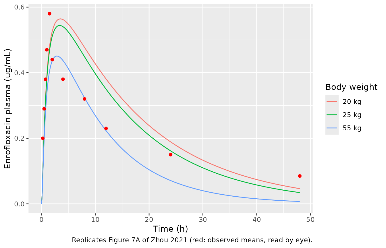
Zhou 2021 validated the plasma prediction against six pigs given 2.5 mg/kg (Figure 7). The pigs weighed 25 +/- 5 kg; because the hepatic metabolic rate constant scales with body weight, the plasma profile is shown at 20 kg (the Table S1 model value), 25 kg (the study mean) and 55 kg (the code default). The observed means were read by eye from Figure 7A by the maintainers and are approximate.
t_pk <- sort(unique(c(seq(0, 2, by = 0.05), seq(2, 48, by = 0.25))))
pk <- bind_rows(
  solve_arm(mod_typ, make_events(20, 2.5, 24, 1, t_pk, "20 kg")),
  solve_arm(mod_typ, make_events(25, 2.5, 24, 1, t_pk, "25 kg")),
  solve_arm(mod_typ, make_events(55, 2.5, 24, 1, t_pk, "55 kg"))
)
fig7_obs <- data.frame(
  time = c(0.25, 0.5, 0.75, 1, 1.5, 2, 4, 8, 12, 24, 48),
  Cc = c(0.20, 0.29, 0.38, 0.47, 0.58, 0.44, 0.38, 0.32, 0.23, 0.15, 0.085)
)
ggplot(pk, aes(time, Cc, colour = arm)) +
  geom_line() +
  geom_point(data = fig7_obs, aes(time, Cc), inherit.aes = FALSE, colour = "red") +
  labs(
    x = "Time (h)", y = "Enrofloxacin plasma (ug/mL)", colour = "Body weight",
    caption = "Replicates Figure 7A of Zhou 2021 (red: observed means, read by eye)."
  )
PKNCA against Table 2
pk_nca <- pk |>
  dplyr::filter(!is.na(Cc)) |>
  dplyr::select(id, time, Cc, arm)
pk_nca <- dplyr::bind_rows(
  pk_nca,
  pk_nca |> dplyr::distinct(id, arm) |> dplyr::mutate(time = 0, Cc = 0)
) |>
  dplyr::distinct(id, arm, time, .keep_all = TRUE) |>
  dplyr::arrange(arm, id, time)
conc_pk <- PKNCA::PKNCAconc(pk_nca, Cc ~ time | arm + id)
dose_pk <- PKNCA::PKNCAdose(
  data.frame(id = 1L, time = 0, amt = 2.5, arm = c("20 kg", "25 kg", "55 kg")),
  amt ~ time | arm + id
)
int_pk <- data.frame(
  start = 0, end = 48, cmax = TRUE, tmax = TRUE, auclast = TRUE,
  half.life = TRUE
)
nca_pk <- PKNCA::pk.nca(PKNCA::PKNCAdata(conc_pk, dose_pk, intervals = int_pk))

published_pk <- tibble::tribble(
  ~arm, ~cmax, ~tmax, ~auclast, ~half.life,
  "25 kg", 0.64, 1.42, 7.96, 12.58
)
cmp_pk <- nlmixr2lib::ncaComparisonTable(
  simulated = nca_pk,
  reference = published_pk,
  by = "arm",
  units = c(cmax = "ug/mL", tmax = "h", auclast = "ug*h/mL", half.life = "h"),
  tolerance_pct = 20
)
knitr::kable(
  cmp_pk,
  caption = paste(
    "Typical pig vs the observed non-compartmental analysis of Zhou 2021",
    "Table 2 (2.5 mg/kg, n = 6, AUC to the last sample at 48 h).",
    "* differs from the reference by >20%."
  )
)| NCA parameter | arm | Reference | Simulated | % diff |
|---|---|---|---|---|
| Cmax (ug/mL) | 25 kg | 0.64 | 0.544 | -15.0% |
| Tmax (h) | 25 kg | 1.42 | 3.5 | +146.5%* |
| AUClast (ug*h/mL) | 25 kg | 7.96 | 10.2 | +28.4%* |
| t½ (h) | 25 kg | 12.6 | 10.8 | -14.1% |
res_pk <- as.data.frame(nca_pk$result)
cmax_25 <- res_pk$PPORRES[res_pk$arm == "25 kg" & res_pk$PPTESTCD == "cmax"]
auc_20 <- res_pk$PPORRES[res_pk$arm == "20 kg" & res_pk$PPTESTCD == "auclast"]
auc_55 <- res_pk$PPORRES[res_pk$arm == "55 kg" & res_pk$PPTESTCD == "auclast"]
stopifnot(
  # A mis-transcribed flow, volume, partition coefficient or dose unit moves
  # Cmax by far more than this.
  abs(cmax_25 / 0.64 - 1) < 0.25,
  # Heavier pigs clear faster (kmet is proportional to WT).
  auc_55 < 0.7 * auc_20
)
At the study weight the typical pig reaches a Cmax within about 15% of the observed mean, but the simulated peak is later (about 3.5 h against the observed 1.42 h) and the exposure to 48 h is about 28% higher than observed. The published curve in Figure 7A peaks at about 1.3 h, earlier than the printed code can produce at any body weight: absorbed drug reaches venous blood only after passing through the liver and mixing into a large, slowly equilibrating rest-of-body compartment (Prest = 8). No combination of the printed parameters and the three documented body weights reproduces Figure 7A (see Errata).
Small-intestinal contents (Section 3.7, Figures 8A and 8C)
Zhou 2021 reports the intestinal-content prediction at 5 mg/kg once daily as AUC24 = 1065.23 ugh/mL, Cmax = 201.07 ug/mL and Tmax = 1.0 h, and AUC24 = 2130 ugh/mL at 10 mg/kg once daily (Section 3.7). Those numbers are not reproduced by the model as printed. The maintainers traced the discrepancy to two differences between the printed code and the run that made the published predictions:
-
The reported “concentration” is the amount in mg.
The code line that converts the intestinal output to mg,
CAImg = AI*MWmg, omits the division by the intestine volume thatCAI = AI/VSiapplies one line earlier. The published sensitivity analysis confirms it: Figure 9 gives a body-weight sensitivity of exactly 1.0 for the intestinal peak, which is what an amount (proportional to the per-kg dose times weight) gives. A true concentration, amount / (0.036 x WT), has a body-weight sensitivity of- Numerically, the published intestinal values therefore equal the
depotstate in mg at the code’sBW = 55kg.
- Numerically, the published intestinal values therefore equal the
-
The run used Ka near 0.25 /h, not 0.55 /h. With Kst
= 2 /h fixed, the intestinal curve is a two-exponential whose slow rate
is
Ka + Kfeces. Figure 8C falls from about 203 at 1.2 h to about 13 at 12 h, a rate of about 0.25 /h; the printed Ka + Kfeces = 0.56 /h would fall to about 0.5 by 12 h.Ka = 0.25 /hreproduces the published Cmax (the reported 201.07 at Tmax = 1.0 h is the curve’s value at 1.0 h; its true peak is 203 at 1.2 h) and AUC24 at both doses to within about 1%. Because the peak depends on Ka and Kfeces only through their sum, the ratio of their sensitivities equals Ka / Kfeces; Figure 9 gives -4.9 / -0.2 = 24.5, matching 0.25 / 0.01 = 25.
The packaged model keeps the printed Ka = 0.55 /h, which
both Table S2 and the code state. The reconstruction below re-sets Ka to
0.25 /h only to show where the published numbers come from.
mod_asrun <- mod_typ |> rxode2::ini(lka = log(0.25))
#> ℹ change initial estimate of `lka` to `-1.38629436111989`

t_int <- sort(unique(c(seq(0, 24, by = 0.1), 1)))
int_arms <- bind_rows(
  solve_arm(mod_typ, make_events(55, 5, 24, 1, t_int, "Printed Ka 0.55, 5 mg/kg QD")),
  solve_arm(mod_typ, make_events(55, 10, 24, 1, t_int, "Printed Ka 0.55, 10 mg/kg QD")),
  solve_arm(mod_asrun, make_events(55, 5, 24, 1, t_int, "Ka 0.25, 5 mg/kg QD")),
  solve_arm(mod_asrun, make_events(55, 10, 24, 1, t_int, "Ka 0.25, 10 mg/kg QD"))
) |>
  dplyr::mutate(Aint = depot) # the published 'ug/mL' is the amount in mg
int_nca <- int_arms |>
  dplyr::filter(!is.na(Aint)) |>
  dplyr::select(id, time, Aint, Cintestine, arm)
dose_int <- data.frame(
  id = 1L, time = 0, amt = 55 * c(5, 10, 5, 10),
  arm = c(
    "Printed Ka 0.55, 5 mg/kg QD", "Printed Ka 0.55, 10 mg/kg QD",
    "Ka 0.25, 5 mg/kg QD", "Ka 0.25, 10 mg/kg QD"
  )
)
int_intervals <- data.frame(start = 0, end = 24, cmax = TRUE, tmax = TRUE, auclast = TRUE)
nca_amt <- PKNCA::pk.nca(PKNCA::PKNCAdata(
  PKNCA::PKNCAconc(int_nca, Aint ~ time | arm + id),
  PKNCA::PKNCAdose(dose_int, amt ~ time | arm + id),
  intervals = int_intervals
))
nca_conc <- PKNCA::pk.nca(PKNCA::PKNCAdata(
  PKNCA::PKNCAconc(int_nca, Cintestine ~ time | arm + id),
  PKNCA::PKNCAdose(dose_int, amt ~ time | arm + id),
  intervals = int_intervals
))
published_int <- tibble::tribble(
  ~arm, ~cmax, ~tmax, ~auclast,
  "Printed Ka 0.55, 5 mg/kg QD", 201.07, 1.0, 1065.23,
  "Printed Ka 0.55, 10 mg/kg QD", NA, NA, 2130,
  "Ka 0.25, 5 mg/kg QD", 201.07, 1.0, 1065.23,
  "Ka 0.25, 10 mg/kg QD", NA, NA, 2130
)
cmp_int <- nlmixr2lib::ncaComparisonTable(
  simulated = nca_amt,
  reference = published_int,
  by = "arm",
  units = c(cmax = "ug/mL", tmax = "h", auclast = "ug*h/mL"),
  tolerance_pct = 20
)
knitr::kable(
  cmp_int,
  caption = paste(
    "Intestinal 'concentration' as reported by Zhou 2021 (the depot amount in",
    "mg at 55 kg; AUC over 0-24 h) against Section 3.7. * differs by >20%."
  )
)| NCA parameter | arm | Reference | Simulated | % diff |
|---|---|---|---|---|
| Cmax (ug/mL) | Printed Ka 0.55, 5 mg/kg QD | 201 | 168 | -16.6% |
| Cmax (ug/mL) | Printed Ka 0.55, 10 mg/kg QD | — | 335 | — |
| Cmax (ug/mL) | Ka 0.25, 5 mg/kg QD | 201 | 203 | +0.8% |
| Cmax (ug/mL) | Ka 0.25, 10 mg/kg QD | — | 405 | — |
| Tmax (h) | Printed Ka 0.55, 5 mg/kg QD | 1 | 0.9 | -10.0% |
| Tmax (h) | Printed Ka 0.55, 10 mg/kg QD | — | 0.9 | — |
| Tmax (h) | Ka 0.25, 5 mg/kg QD | 1 | 1.2 | +20.0%* |
| Tmax (h) | Ka 0.25, 10 mg/kg QD | — | 1.2 | — |
| AUClast (ug*h/mL) | Printed Ka 0.55, 5 mg/kg QD | 1070 | 491 | -53.9%* |
| AUClast (ug*h/mL) | Printed Ka 0.55, 10 mg/kg QD | 2130 | 981 | -53.9%* |
| AUClast (ug*h/mL) | Ka 0.25, 5 mg/kg QD | 1070 | 1050 | -1.0% |
| AUClast (ug*h/mL) | Ka 0.25, 10 mg/kg QD | 2130 | 2110 | -1.0% |
The true concentration in the small-intestinal contents,
Cintestine, is the same at any body weight:
as.data.frame(nca_conc$result) |>
  dplyr::filter(PPTESTCD %in% c("cmax", "auclast")) |>
  dplyr::select(arm, PPTESTCD, PPORRES) |>
  tidyr::pivot_wider(names_from = PPTESTCD, values_from = PPORRES) |>
  dplyr::rename(
    "Arm" = arm, "Cmax (ug/mL)" = cmax, "AUC0-24 (ug*h/mL)" = auclast
  ) |>
knitr::kable(digits = 1, caption = "Concentration in the small-intestinal contents (Cintestine).")| Arm | AUC0-24 (ug*h/mL) | Cmax (ug/mL) |
|---|---|---|
| Ka 0.25, 10 mg/kg QD | 1065.5 | 204.7 |
| Ka 0.25, 5 mg/kg QD | 532.7 | 102.4 |
| Printed Ka 0.55, 10 mg/kg QD | 495.5 | 169.3 |
| Printed Ka 0.55, 5 mg/kg QD | 247.7 | 84.6 |
res_amt <- as.data.frame(nca_amt$result)
get_amt <- function(arm, code) res_amt$PPORRES[res_amt$arm == arm & res_amt$PPTESTCD == code]
a1_asrun <- int_arms$Aint[int_arms$arm == "Ka 0.25, 5 mg/kg QD" & int_arms$time == 1]
stopifnot(
  # The Ka = 0.25 reconstruction reproduces Section 3.7 (Cmax read at the
  # reported Tmax of 1.0 h; AUC24 at 5 and 10 mg/kg).
  abs(a1_asrun / 201.07 - 1) < 0.01,
  abs(get_amt("Ka 0.25, 5 mg/kg QD", "auclast") / 1065.23 - 1) < 0.02,
  abs(get_amt("Ka 0.25, 10 mg/kg QD", "auclast") / 2130 - 1) < 0.02,
  # The printed Ka does not: its AUC24 is less than half the published value.
  get_amt("Printed Ka 0.55, 5 mg/kg QD", "auclast") < 0.5 * 1065.23
)
t_bid <- sort(unique(c(seq(0, 144, by = 0.1))))
bid <- bind_rows(
  solve_arm(mod_typ, make_events(55, 5, 12, 10, t_bid, "Printed Ka 0.55")),
  solve_arm(mod_asrun, make_events(55, 5, 12, 10, t_bid, "Ka 0.25"))
)
fig8_obs <- data.frame(
  time = c(1, 109, 112, 120, 132),
  Aint = c(183, 256, 102, 12, 1)
)
ggplot(bid, aes(time, depot, colour = arm)) +
  geom_line() +
  geom_point(data = fig8_obs, aes(time, Aint), inherit.aes = FALSE, colour = "red", shape = 17) +
  labs(
    x = "Time (h)", y = "Intestinal output as published (ug/mL = depot amount, mg)",
    colour = NULL,
    caption = paste(
      "Replicates Figure 8A of Zhou 2021: 5 mg/kg twice daily for 5 days, 55 kg.",
      "Red: observed means, read by eye.",
      sep = "\n"
    )
  )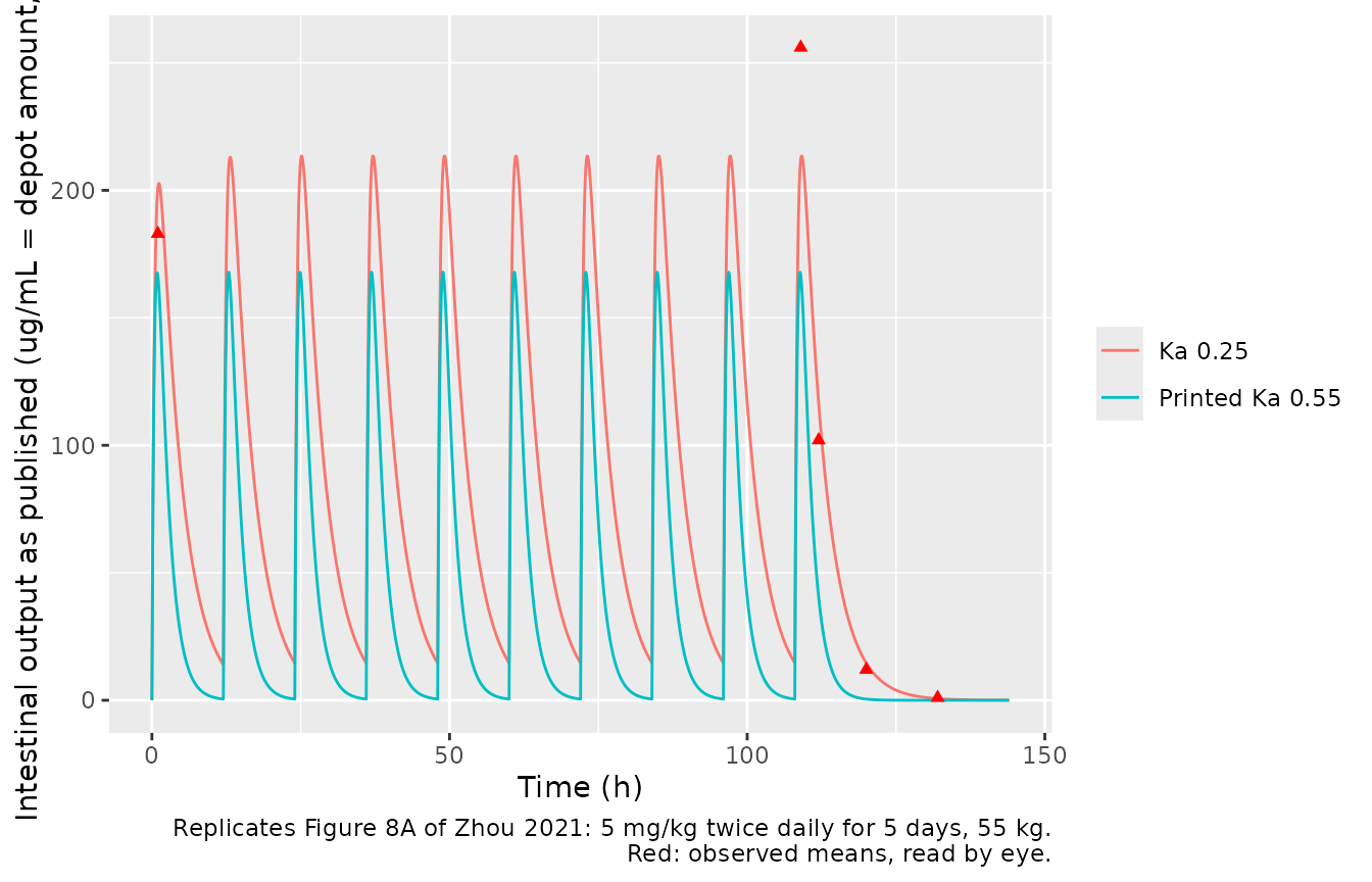
With Ka = 0.25 /h the profile matches Figure 8A (peaks near 213 at
steady state, troughs near 15). The observed intestinal data were
measured in ug/mL of contents, so their agreement with an amount in mg
is a coincidence of the 55 kg body weight; the physically consistent
prediction, Cintestine, peaks near 85 ug/mL (printed Ka) or
102 ug/mL (Ka = 0.25).
Parameter sensitivity (Figure 9)
Figure 9 reports normalised sensitivity coefficients (NSC = relative change in the intestinal peak / relative change in the parameter, for a 1% increase) of 1.0 for body weight, -4.9 for Ka, -0.2 for Kfeces and -0.1 for Kst.
nsc_peak <- function(model, output, param_values) {
  ev <- make_events(55, 5, 24, 1, seq(0, 24, by = 0.01), "nsc")
  base <- max(solve_arm(model, ev)[[output]])
  out <- c()
  ev_bw <- make_events(55 * 1.01, 5, 24, 1, seq(0, 24, by = 0.01), "nsc")
  out["BW"] <- (max(solve_arm(model, ev_bw)[[output]]) / base - 1) / 0.01
  for (p in names(param_values)) {
    new_ini <- setNames(list(log(param_values[[p]] * 1.01)), p)
    m2 <- rxode2::ini(model, new_ini)
    out[p] <- (max(solve_arm(m2, ev)[[output]]) / base - 1) / 0.01
  }
  out
}
nsc <- rbind(
  "Amount (as published), Ka 0.25" = nsc_peak(mod_asrun, "depot", list(lka = 0.25, lkfec = 0.01, lkst = 2)),
  "Concentration, Ka 0.25" = nsc_peak(mod_asrun, "Cintestine", list(lka = 0.25, lkfec = 0.01, lkst = 2)),
  "Amount, printed Ka 0.55" = nsc_peak(mod_typ, "depot", list(lka = 0.55, lkfec = 0.01, lkst = 2)),
  "Published (Figure 9)" = c(1.0, -4.9, -0.2, -0.1)
)
#> ℹ change initial estimate of `lka` to `-1.37634403026672`
#> ℹ change initial estimate of `lkfec` to `-4.59521985513492`
#> ℹ change initial estimate of `lkst` to `0.703097511413113`
#> ℹ change initial estimate of `lka` to `-1.37634403026672`
#> ℹ change initial estimate of `lkfec` to `-4.59521985513492`
#> ℹ change initial estimate of `lkst` to `0.703097511413113`
#> ℹ change initial estimate of `lka` to `-0.587886669902452`
#> ℹ change initial estimate of `lkfec` to `-4.59521985513492`
#> ℹ change initial estimate of `lkst` to `0.703097511413113`
colnames(nsc) <- c("BW", "Ka", "Kfeces", "Kst")
knitr::kable(nsc, digits = 2, caption = "Normalised sensitivity of the intestinal peak.")| BW | Ka | Kfeces | Kst | |
|---|---|---|---|---|
| Amount (as published), Ka 0.25 | 1 | -0.19 | -0.01 | 0.2 |
| Concentration, Ka 0.25 | 0 | -0.19 | -0.01 | 0.2 |
| Amount, printed Ka 0.55 | 1 | -0.29 | -0.01 | 0.3 |
| Published (Figure 9) | 1 | -4.90 | -0.20 | -0.1 |
stopifnot(
  abs(nsc["Amount (as published), Ka 0.25", "BW"] - 1) < 0.05,
  abs(nsc["Concentration, Ka 0.25", "BW"]) < 0.05,
  nsc["Amount (as published), Ka 0.25", "Ka"] < 0
)
The body-weight coefficient of 1.0 identifies the published intestinal output as an amount. The signs of the Ka and Kfeces coefficients agree with the paper and their ratio is close to the published one, but their magnitudes do not: for this two-exponential curve the peak cannot change by more than about 1% per 1% change in a rate constant, so the published -4.9 cannot be reproduced by any setting of the model. The published Kst coefficient also has the opposite sign.
Mass balance
The code carries an explicit mass-balance check (Bal).
Every state here is a drug amount in mg, so the sum over all of them,
including the urine, metabolism and faeces sinks, must equal the dose at
every time. Dropping the metabolism sink from the sum (a mutation
control) must break the balance.
t_mb <- c(0, 0.5, 1, 2, 4, 8, 24, 48, 96)
mb <- solve_arm(
  mod_typ, make_events(25, 2.5, 24, 1, t_mb, "mb"),
  atol = 1e-12, rtol = 1e-10
)
state_cols <- c(
  "stomach", "depot", "a_liver", "a_kidney", "a_muscle", "a_fat", "a_remainder",
  "a_pulmonary", "a_venous", "a_arterial", "a_urine", "a_metabolized", "a_feces"
)
dose_mg <- 2.5 * 25
total <- rowSums(mb[, state_cols])
mutant <- rowSums(mb[, setdiff(state_cols, "a_metabolized")])
stopifnot(
  max(abs(total / dose_mg - 1)) < 1e-6,
  max(abs(mutant / dose_mg - 1)) > 0.1
)
knitr::kable(
  data.frame(
    time = mb$time, total_mg = total, urine = mb$a_urine,
    metabolized = mb$a_metabolized, feces = mb$a_feces
  ),
  digits = 3,
  caption = "Mass balance after 2.5 mg/kg (62.5 mg) at 25 kg."
)| time | total_mg | urine | metabolized | feces |
|---|---|---|---|---|
| 0.0 | 62.5 | 0.000 | 0.000 | 0.000 |
| 0.5 | 62.5 | 0.097 | 0.452 | 0.104 |
| 1.0 | 62.5 | 0.462 | 1.631 | 0.289 |
| 2.0 | 62.5 | 1.598 | 4.352 | 0.618 |
| 4.0 | 62.5 | 4.280 | 8.828 | 0.951 |
| 8.0 | 62.5 | 9.282 | 15.014 | 1.099 |
| 24.0 | 62.5 | 20.612 | 27.573 | 1.116 |
| 48.0 | 62.5 | 25.557 | 33.021 | 1.116 |
| 96.0 | 62.5 | 26.832 | 34.425 | 1.116 |
With the printed rate constants,
Ka / (Ka + Kfeces) = 98% of the oral dose is absorbed;
hepatic metabolism is the main route of elimination.
Intravenous route
The code also accepts an intravenous dose into venous blood
(a_venous); the Zhou 2021 application did not use it.
iv <- solve_arm(mod_typ, make_events(25, 2.5, 24, 1, t_pk, "IV 2.5 mg/kg", cmt = "a_venous"))
ggplot(iv, aes(time, Cc)) +
  geom_line() +
  scale_y_log10() +
  labs(x = "Time (h)", y = "Enrofloxacin plasma (ug/mL)", caption = "Single 2.5 mg/kg intravenous bolus, 25 kg.")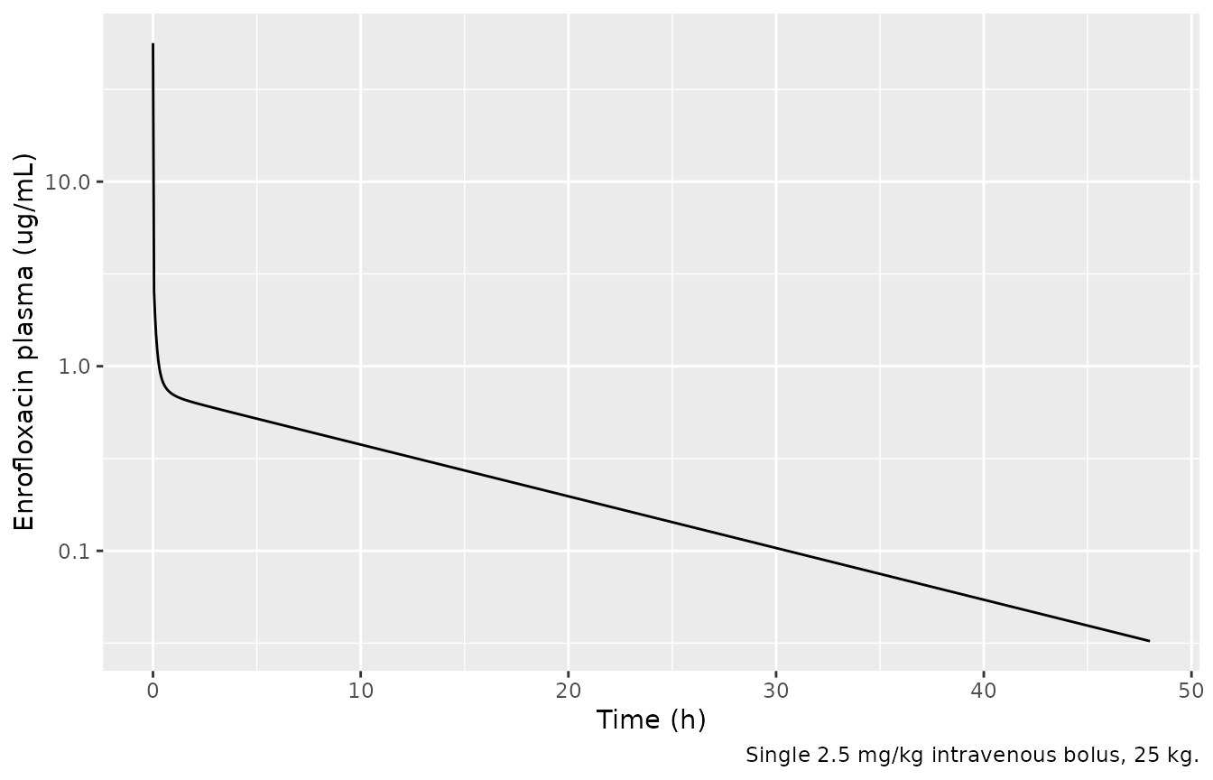
Assumptions and deviations
-
The code is the model. The supplementary acslXtreme
code and Tables S1 and S2 agree on every value used here, except body
weight (below); the rest-of-body partition coefficient
Prest = 8is in the code only. -
Absorption rate constant. The packaged model uses
the printed
Ka = 0.55 /h. The intestinal predictions of Section 3.7 and Figure 8 were evidently made withKanear 0.25 /h (reconstructed above to within 1% on Cmax and 2% on AUC24); that value is printed nowhere, so it is not used as the default. A user who wants the published intestinal predictions can setrxode2::ini(mod, lka = log(0.25)). -
Intestinal output. The published intestinal
“concentration” (ug/mL) is the amount of drug in the small-intestinal
contents in mg, because the code’s mg-conversion line
CAImg = AI*MWmgomits the division by the intestine volume. The model exposes the physically consistent concentrationCintestine = depot / (0.036 * WT); the published quantity is thedepotstate. Since the manual re-calibration of the intestine volume (0.036 instead of 0.0126) cannot have changed an amount, it did not influence the published intestinal fit. - Figure 7 not reproduced. The plasma curve in Figure 7A peaks earlier (about 1.3 h) than the printed code allows at any of the three documented body weights (20, 25 and 55 kg). No parameter was tuned toward it.
- Figure 9 magnitudes not reproduced. The published Ka coefficient (-4.9) is outside what the model structure allows; only the body-weight coefficient and the Ka / Kfeces ratio are consistent.
-
Body weight. The code sets
BW = 55kg (“study-specific; the actual value in present study”), which the intestinal reconstruction needs; Table S1 prints 20 kg and the plasma-study pigs weighed 25 +/- 5 kg. Because the hepatic metabolic rate constant isKmC * BW, hepatic clearance grows as body weight squared, so the plasma profile depends on weight even with a per-kg dose. The model default is 55 kg. - Molecular-weight conversion. The code works in umol, converting with the rounded constants 2.78 umol/mg and 0.36 mg/umol, whose product is 1.0008. The model works in mg throughout, so its concentrations are 0.08% below the code’s.
-
Routes left out. The code’s intramuscular and
subcutaneous branches (
Kim,Ksc) are set to 0 in Zhou 2021 (Table S2 ‘model value 0.0’), which disables them, so they are not encoded. The ciprofloxacin (metabolite) partition coefficients in the code are declared but never used by any equation; the metabolite was not modelled. -
Dosing. The code delivers each oral dose into the
stomach as a 0.001-h pulse; the model uses a bolus into
stomach. -
Residual error. Zhou 2021 reports none;
propSdandpropSd_Cintestineare fixed placeholders so the model is a complete nlmixr2 object, and are not estimates. - Errata. Europe PMC lists no correction notice for Zhou 2021 (PMID 33922109) as of 2026-09-28.