Raltegravir (Bukkems 2021)
Source:vignettes/articles/Bukkems_2021_raltegravir.Rmd
Bukkems_2021_raltegravir.RmdModel and source
- Citation: Bukkems VE, Post TM, Colbers AP, Burger DM, Svensson EM. A population pharmacokinetics analysis assessing the exposure of raltegravir once-daily 1200 mg in pregnant women living with HIV. CPT Pharmacometrics Syst Pharmacol. 2021;10(2):161-172. doi:10.1002/psp4.12586.
- Description: Two-compartment population PK model for oral raltegravir in a pooled cohort of 221 adults (healthy volunteers, non-pregnant adults living with HIV, and pregnant women living with HIV) across the 400 mg BID, 800 mg QD, and 1200 mg QD (two 600 mg tablets) regimens (Bukkems 2021). Absorption is modelled as a chain of four sequential first-order compartments: depot -> transit1 -> transit2 -> transit3 -> central, with the first three transitions governed by a shared rate constant ktr = 3 / mat (paper’s mean transit time MAT parameter) and the final transit3 -> central transition governed by a separate first-order absorption rate constant ka. Disposition is a two-compartment linear model with apparent central and peripheral volumes and apparent clearance and inter-compartmental clearance. Body weight enters as allometric scaling with fixed exponents 0.75 on CL and Q and 1.0 on Vc and Vp, referenced to 70 kg. Six covariate-parameter relationships are retained in the final model: FED on MAT (+160% with any food), CONMED_ATAZANAVIR on CL (-17%), FORM_RAL_600 on F (+21%), FED_LOWFAT on F (-46%), PREG on F (-49%), and CONMED_EFV on F (-17%). Inter-individual variability is a diagonal eta on Vc plus a correlated 3-parameter block on CL, Q, and Vp with the CL-Vp off-diagonal fixed to zero. Residual error is a proportional model with a time-varying magnitude that switches at 3 h after dose (43.5% CV before, 29.0% CV after, tracking the paper’s empirical time-varying residual). The paper’s inter-occasion variability on F and MAT and its additional eta on the residual magnitude are omitted from this packaged model; see the validation vignette Assumptions and deviations section.
- Article: https://doi.org/10.1002/psp4.12586
Population
Bukkems 2021 pooled 11 raltegravir PK studies (references 8, 10, 14-21 in the source), yielding 221 individuals and 4016 sampling points after exclusions. Constituent studies represented healthy adults on the 400 mg twice-daily (BID) regimen, healthy adults on the 1200 mg once-daily (QD, given as two 600 mg tablets) regimen, HIV-infected non-pregnant adults on either regimen (with various concomitant antiretrovirals including atazanavir and efavirenz), and 22 HIV-infected pregnant women in the third trimester (target gestational age 33 weeks) on the 400 mg BID regimen. Table 1 of the source gives per-study demographics; the pooled cohort spans ages 18-75 years and weights 43-111 kg, and includes fasted, low-fat-meal, moderate-fat-meal, and (a limited number of) high-fat-meal dose records. Two additional HIV-infected pregnant women were sampled during the third trimester and postpartum on 1200 mg QD raltegravir as clinical cases; they were compared against the model’s simulation predictions but were not included in the model-building dataset.
The same population information is available programmatically via
readModelDb("Bukkems_2021_raltegravir")()$population.
Source trace
The per-parameter origin is recorded as an in-file comment next to
each ini() entry in
inst/modeldb/specificDrugs/Bukkems_2021_raltegravir.R. The
table below collects them in one place for review.
| Equation / parameter | Value | Source location |
|---|---|---|
lka |
log(0.741 h^-1) | Table 2: Ka = 0.741 h^-1 (RSE 2%) |
lmat (fasted MAT) |
log(0.336 h) | Table 2: MAT = 0.336 h fasted (RSE 8%) |
lvc (Vc/F @ 70 kg) |
log(44.3 L) | Table 2: V_c/F = 44.3 L (RSE 7%) |
lcl (CL/F @ 70 kg) |
log(55.8 L/h) | Table 2: CL/F = 55.8 L/h (RSE 5%) |
lq (Q/F @ 70 kg) |
log(5.68 L/h) | Table 2: Q/F = 5.68 L/h (RSE 7%) |
lvp (Vp/F @ 70 kg) |
log(92.8 L) | Table 2: V_p/F = 92.8 L (RSE 9%) |
lfdepot (F) |
fixed(log(1)) | Table 2 footnote c: F = 1 fixed reference |
e_wt_cl (CL, Q exponent) |
fixed(0.75) | Methods, allometric-scaling paragraph |
e_wt_vc (Vc, Vp exponent) |
fixed(1.0) | Methods, allometric-scaling paragraph |
e_fed_mat |
+1.6 | Table 2: Factor change in MAT fed = 1.6 |
e_atazanavir_cl |
-0.17 | Table 2: Factor change in CL with atazanavir |
e_ral_600_fdepot |
+0.209 | Table 2: Factor change in F 600 mg formulation |
e_lowfat_fdepot |
-0.459 | Table 2: Factor change in F low-fat meal |
e_preg_fdepot |
-0.487 | Table 2: Factor change in F pregnancy |
e_efv_fdepot |
-0.167 | Table 2: Factor change in F efavirenz co-admin |
| IIV Vc/F (69.7% CV) | var = 0.39596 | Table 2: IIV V_c/F = 69.7% (RSE 14%) |
| IIV CL, Q, Vp block | var 0.07862 / 0.41292 / 0.84462 | Table 2: IIV CL/F 28.6%, Q/F 71.5%, Vp/F 115.2% |
| corr(CL, Q) | 0.18 -> cov 0.03243 | Table 2: correlation coefficient with Q/F = 0.18 |
| corr(Q, Vp) | 0.59 -> cov 0.34843 | Table 2: correlation coefficient with V_p/F = 0.59 |
| corr(CL, Vp) | 0 (fixed) | Supporting Information S4 $OMEGA BLOCK(3) explicit 0 |
propSd_early (PTAD <= 3 h) |
0.435 | Table 2: prop residual <= 3 h = 43.5% (RSE 3%) |
propSd_late (PTAD > 3 h) |
0.290 | Table 2: prop residual > 3 h = 29.0% (RSE 2%) |
| Absorption ODE structure | depot -> t1 -> t2 -> t3 -> central via ktr, ktr, ktr, ka | Figure 1 and Supporting Information S4 $DES |
| Two-compartment disposition | central <-> peripheral1 (Q/Vc, Q/Vp) | Figure 1 and Supporting Information S4 $DES |
| ktr = 3 / mat | derived | Supporting Information S4 $PK line KTR = 3/AMRT
|
Virtual cohort
The paper’s Monte-Carlo simulations resample covariate distributions from 186 pregnant and postpartum women in the European PANNA study, adding 10 % noise. The public source does not release those covariates; the vignette instead constructs a simple virtual cohort with body weight sampled uniformly across the pooled study range (50-100 kg) and applies each of the six meal-by-pregnancy scenarios to the same 100 subjects. The typical-value AUC and Ctrough comparison against Bukkems 2021 Table 3 is insensitive to the exact weight distribution because the paper’s Table 3 headline numbers were generated at typical parameters (see “Assumptions and deviations” below).
set.seed(42)

n_per_scenario <- 100L

scenarios <- tibble::tribble(
  ~cohort,                       ~PREG, ~FED, ~FED_LOWFAT,
  "Non-pregnant, fasted",            0,    0,          0,
  "Non-pregnant, low-fat meal",      0,    1,          1,
  "Non-pregnant, moderate-fat meal", 0,    1,          0,
  "Pregnant, fasted",                1,    0,          0,
  "Pregnant, low-fat meal",          1,    1,          1,
  "Pregnant, moderate-fat meal",     1,    1,          0
)

make_scenario <- function(cohort, PREG, FED, FED_LOWFAT, id_offset) {
  # 1200 mg QD dosed as two 600 mg tablets for 14 days (steady state);
  # observations dense over the last dosing interval so PKNCA can compute
  # steady-state AUC0-24h and Ctrough at 24 h.
  ids <- id_offset + seq_len(n_per_scenario)
  wt  <- runif(n_per_scenario, min = 50, max = 100)

  cov <- tibble::tibble(
    id                = ids,
    WT                = wt,
    PREG              = as.integer(PREG),
    CONMED_ATAZANAVIR = 0L,
    CONMED_EFV        = 0L,
    FORM_RAL_600      = 1L,
    FED               = as.integer(FED),
    FED_LOWFAT        = as.integer(FED_LOWFAT),
    cohort            = cohort
  )

  doses <- tidyr::expand_grid(
    id   = ids,
    time = seq(0, by = 24, length.out = 14)
  ) |>
    dplyr::mutate(
      amt  = 1200,
      evid = 1L,
      cmt  = "depot"
    )

  # Observations on the LAST dosing interval (312-336 h) so that PKNCA sees
  # the steady-state 24-h window. cmt is the ODE-state name "central".
  obs <- tidyr::expand_grid(
    id   = ids,
    time = c(312, 312.5, 313, 314, 315, 316, 318,
             320, 322, 324, 326, 328, 330, 333, 336)
  ) |>
    dplyr::mutate(
      amt  = NA_real_,
      evid = 0L,
      cmt  = "central"
    )

  ev <- dplyr::bind_rows(doses, obs) |>
    dplyr::arrange(id, time, dplyr::desc(evid)) |>
    dplyr::left_join(cov, by = "id")

  ev
}

events <- dplyr::bind_rows(
  make_scenario("Non-pregnant, fasted",            0, 0, 0, id_offset =   0L),
  make_scenario("Non-pregnant, low-fat meal",      0, 1, 1, id_offset = 100L),
  make_scenario("Non-pregnant, moderate-fat meal", 0, 1, 0, id_offset = 200L),
  make_scenario("Pregnant, fasted",                1, 0, 0, id_offset = 300L),
  make_scenario("Pregnant, low-fat meal",          1, 1, 1, id_offset = 400L),
  make_scenario("Pregnant, moderate-fat meal",     1, 1, 0, id_offset = 500L)
)

stopifnot(!anyDuplicated(unique(events[, c("id", "time", "evid")])))

nrow(events)
#> [1] 17400
Simulation
The paper’s Table 3 headline numbers were generated without residual
error and with 3000 individuals per scenario; here we mirror that by
simulating with between-subject variability (IIV block on CL/Q/Vp and
diagonal IIV on Vc) and 100 subjects per scenario, then computing
geometric means. Residual error is carried but zeroed on plots
(rxode2::zeroRe() is not used because IIV is the main
variability of interest).
mod <- readModelDb("Bukkems_2021_raltegravir")

sim <- rxode2::rxSolve(
  mod,
  events = events,
  keep   = c("cohort", "PREG", "FED", "FED_LOWFAT", "FORM_RAL_600", "WT")
) |>
  as.data.frame() |>
  # Re-express time relative to the start of the terminal dose so plots
  # and NCA windows read 0-24 h rather than 312-336 h.
  dplyr::mutate(time_ss = time - 312)
#> ℹ parameter labels from comments will be replaced by 'label()'
Replicate published figures
# Figure 2 of Bukkems 2021 shows a VPC of the observed vs simulated raltegravir
# concentration-time profile; the observed data are not publicly available, so
# we show the model-predicted median and 5th / 95th percentiles as a typical-
# value envelope by scenario.
sim |>
  dplyr::filter(time_ss >= 0, !is.na(Cc)) |>
  dplyr::group_by(cohort, time_ss) |>
  dplyr::summarise(
    Q05 = quantile(Cc, 0.05, na.rm = TRUE),
    Q50 = quantile(Cc, 0.50, na.rm = TRUE),
    Q95 = quantile(Cc, 0.95, na.rm = TRUE),
    .groups = "drop"
  ) |>
  ggplot(aes(time_ss, Q50)) +
  geom_ribbon(aes(ymin = Q05, ymax = Q95), alpha = 0.20) +
  geom_line() +
  facet_wrap(~ cohort, ncol = 3) +
  scale_y_log10() +
  labs(x = "Time since last dose (h)",
       y = "Raltegravir Cc (mg/L)",
       title = "Simulated steady-state raltegravir Cc after 1200 mg QD",
       caption = "Model-predicted median and 5th / 95th percentiles by scenario. Compare with Figure 2 of Bukkems 2021.")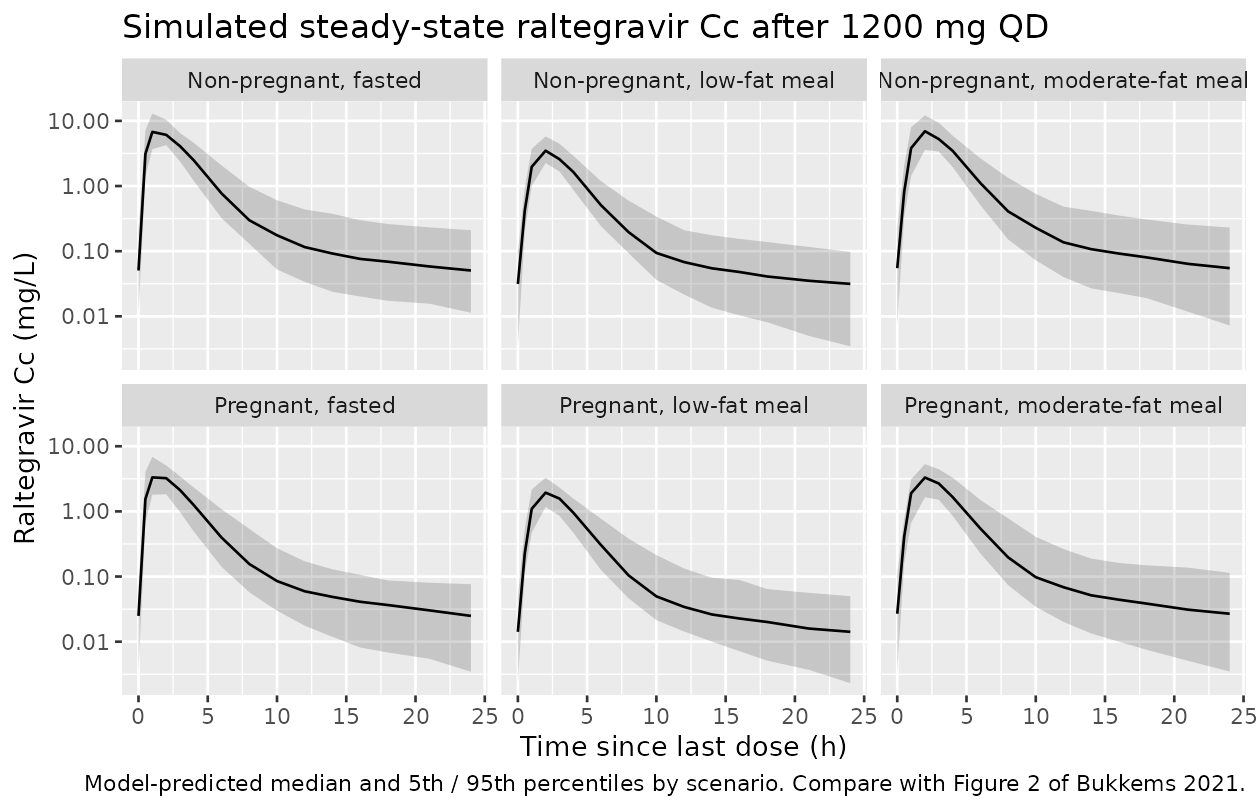
PKNCA validation
We compute steady-state Cmax, Tmax, AUC0-24h, and Ctrough per subject and per scenario, then geometric-mean-summarise by scenario for the side-by-side comparison against Bukkems 2021 Table 3.
sim_nca <- sim |>
  dplyr::filter(time_ss >= 0, !is.na(Cc)) |>
  dplyr::transmute(id, time = time_ss, Cc, treatment = cohort)

# Guarantee a time = 0 row per (id, treatment); Cc at time=0 (start of the
# terminal dosing interval) is the previous Ctrough of a steady-state profile.
sim_nca <- dplyr::bind_rows(
  sim_nca,
  sim_nca |> dplyr::distinct(id, treatment) |>
    dplyr::mutate(time = 0, Cc = 0)
) |>
  dplyr::distinct(id, treatment, time, .keep_all = TRUE) |>
  dplyr::arrange(id, treatment, time)

conc_obj <- PKNCA::PKNCAconc(sim_nca, Cc ~ time | treatment + id)

dose_df <- events |>
  dplyr::filter(evid == 1L, time == max(time[evid == 1L])) |>
  dplyr::transmute(id, time = 0, amt, treatment = cohort)

dose_obj <- PKNCA::PKNCAdose(dose_df, amt ~ time | treatment + id)

intervals <- data.frame(
  start   = 0,
  end     = 24,
  cmax    = TRUE,
  tmax    = TRUE,
  auclast = TRUE,
  ctrough = TRUE
)

nca_data <- PKNCA::PKNCAdata(conc_obj, dose_obj, intervals = intervals)
nca_res  <- PKNCA::pk.nca(nca_data)
gm_ci <- function(x, na.rm = TRUE) {
  x <- x[!is.na(x) & x > 0]
  if (!length(x)) return(tibble::tibble(GM = NA_real_, LCL = NA_real_, UCL = NA_real_))
  lx <- log(x); n <- length(lx)
  se <- sd(lx) / sqrt(n)
  tibble::tibble(
    GM  = exp(mean(lx)),
    LCL = exp(mean(lx) - 1.96 * se),
    UCL = exp(mean(lx) + 1.96 * se)
  )
}

nca_wide <- as.data.frame(nca_res$result) |>
  dplyr::select(treatment, id, PPTESTCD, PPORRES) |>
  tidyr::pivot_wider(names_from = PPTESTCD, values_from = PPORRES)

nca_summary <- nca_wide |>
  dplyr::group_by(treatment) |>
  dplyr::summarise(
    n          = dplyr::n(),
    cmax_gm    = gm_ci(cmax)$GM,
    auclast_gm = gm_ci(auclast)$GM,
    ctrough_gm = gm_ci(ctrough)$GM,
    .groups    = "drop"
  )

nca_summary |>
  dplyr::rename(
    "Scenario"                = treatment,
    "N"                       = n,
    "Cmax (mg/L)"             = cmax_gm,
    "AUC0-24 (mg*h/L)"        = auclast_gm,
    "Ctrough at 24 h (mg/L)"  = ctrough_gm
  ) |>
  knitr::kable(
    digits  = 3,
    caption = "Model-predicted geometric means at steady state (1200 mg QD, 14 days)."
)| Scenario | N | Cmax (mg/L) | AUC0-24 (mg*h/L) | Ctrough at 24 h (mg/L) |
|---|---|---|---|---|
| Non-pregnant, fasted | 100 | 7.284 | 24.768 | 0.048 |
| Non-pregnant, low-fat meal | 100 | 3.562 | 12.797 | 0.024 |
| Non-pregnant, moderate-fat meal | 100 | 6.889 | 25.789 | 0.050 |
| Pregnant, fasted | 100 | 3.713 | 12.364 | 0.020 |
| Pregnant, low-fat meal | 100 | 1.968 | 7.144 | 0.013 |
| Pregnant, moderate-fat meal | 100 | 3.271 | 12.442 | 0.024 |
Comparison against Bukkems 2021 Table 3
Table 3 of the source paper reports the “Simulations with typical parameter estimates (n individuals = 3000)” for the same six scenarios. The GM values below are the paper’s typical-value simulations; the 95 % CI in Table 3 is built from between-subject variability. We compare geometric means (the paper’s headline metric).
published <- tibble::tribble(
  ~treatment,                        ~auclast, ~ctrough,
  "Non-pregnant, fasted",              25.45,   0.047,
  "Non-pregnant, low-fat meal",        13.76,   0.028,
  "Non-pregnant, moderate-fat meal",   25.45,   0.052,
  "Pregnant, fasted",                  13.06,   0.024,
  "Pregnant, low-fat meal",             7.06,   0.014,
  "Pregnant, moderate-fat meal",       13.06,   0.027
)

compare_tbl <- nca_summary |>
  dplyr::transmute(
    treatment,
    "AUC0-24 sim (mg*h/L)" = round(auclast_gm, 2),
    "Ctrough sim (mg/L)"   = round(ctrough_gm, 3)
  ) |>
  dplyr::left_join(
    published |>
      dplyr::rename(
        "AUC0-24 published (mg*h/L)" = auclast,
        "Ctrough published (mg/L)"   = ctrough
      ),
    by = "treatment"
  ) |>
  dplyr::mutate(
    "AUC pct diff" = round(
      100 * (`AUC0-24 sim (mg*h/L)` - `AUC0-24 published (mg*h/L)`) /
        `AUC0-24 published (mg*h/L)`, 1),
    "Ctrough pct diff" = round(
      100 * (`Ctrough sim (mg/L)` - `Ctrough published (mg/L)`) /
        `Ctrough published (mg/L)`, 1)
  ) |>
  dplyr::rename("Scenario" = treatment)

knitr::kable(
  compare_tbl,
  caption = "Simulated vs published (Bukkems 2021 Table 3) steady-state AUC and Ctrough. Percent difference reported for each scenario; agreement within ~20 % is expected given the simplified 100-subject virtual cohort here vs the paper's 3000-subject Monte-Carlo procedure."
)| Scenario | AUC0-24 sim (mg*h/L) | Ctrough sim (mg/L) | AUC0-24 published (mg*h/L) | Ctrough published (mg/L) | AUC pct diff | Ctrough pct diff |
|---|---|---|---|---|---|---|
| Non-pregnant, fasted | 24.77 | 0.048 | 25.45 | 0.047 | -2.7 | 2.1 |
| Non-pregnant, low-fat meal | 12.80 | 0.024 | 13.76 | 0.028 | -7.0 | -14.3 |
| Non-pregnant, moderate-fat meal | 25.79 | 0.050 | 25.45 | 0.052 | 1.3 | -3.8 |
| Pregnant, fasted | 12.36 | 0.020 | 13.06 | 0.024 | -5.4 | -16.7 |
| Pregnant, low-fat meal | 7.14 | 0.013 | 7.06 | 0.014 | 1.1 | -7.1 |
| Pregnant, moderate-fat meal | 12.44 | 0.024 | 13.06 | 0.027 | -4.7 | -11.1 |
Assumptions and deviations
-
IOV (inter-occasion variability) is not encoded.
Bukkems 2021 estimates IOV on F (112.1 % CV for the 400 mg tablet,
reduced to 31.6 % CV for the 600 mg tablet via the
NEW-formulation modifier) and on the mean transit time (140.5 % CV). The paper’s IOV structure uses five occasions defined by study-specificFLAGDandCURVEindicators (Supporting Information S4$PKblock); those record-level occasion indicators are not defined for the general-use simulation contexts targeted by this model file. The packaged model omits IOV, following theAndrews_2017_tacrolimus/Brooks_2021_tacrolimusprecedent. Downstream users who want IOV in simulations can add anOCCcovariate and per-occasion etas in rxode2. -
Log-normal per-subject scaling of the proportional residual
error is not encoded. Table 2 reports “IIV residual error, %” =
25.6 % CV, which the NONMEM control stream implements as an ETA on the
residual magnitude
(
Y = IPRED + IPRED * ERR * EXP(ETA(13))). nlmixr2’s proportional error syntax (Cc ~ prop(propSd)) does not natively support a per-subject scaling on the residual SD. The packaged model uses only the two time-varying magnitudes (43.5 % CV for time-after-dose <= 3 h, 29.0 % CV for > 3 h); the per-subject scaling is a secondary variability layer that modestly widens simulated 95 % concentration intervals in the paper. -
High-fat meal effect is not encoded. Bukkems 2021
reports that simulations with high-fat conditions were not carried
through because “the model did not perform sufficiently under these
conditions and it was not believed to be a commonly occurring meal type
(~1000 kcal and 50 % fat)”. The
FED_HIGHFATcanonical is therefore intentionally NOT wired into the model file; only fasted / low-fat / (any-food-including-)moderate-fat conditions are supported. - Weight scaling for pregnant women uses postpartum weight. The source paper uses postpartum weight (or 0.93 x third-trimester weight when postpartum is missing) as the allometric size descriptor for pregnant subjects, because applicability of allometric scaling in pregnancy has not been established. In this vignette’s virtual cohort, WT is a single per- subject value; when simulating pregnant subjects, treat WT as their postpartum (or postpartum-imputed) weight, not their third-trimester weight.
- Bioavailability F is fixed at 1 (typical value). No intravenous raltegravir data were available to estimate absolute F; F = 1 is the structural anchor and the covariate multipliers on F are all reported as relative shifts from that anchor. Simulated AUC / Ctrough scale linearly with any user-imposed absolute-F factor.
- Virtual cohort covariates are approximated. The paper’s simulations resample covariates from 186 European PANNA subjects; that dataset is not public. This vignette uses a simple uniform WT(50-100 kg) draw for the virtual cohort and holds concomitant atazanavir / efavirenz at 0. Any application requiring the paper’s exact covariate joint distribution should build the cohort from the operational study’s own covariate data.
-
PKNCA time-window choice. The Table 3 comparison
uses steady-state 0-24 h AUC (
auclaston a 24-h grid). The paper reports geometric-mean AUC and Ctrough at 24 h; both align with the PKNCA output labelsauclastandctroughon the terminal 24-h dosing interval of a 14-day QD schedule.