Piperacillin/tazobactam in sepsis and septic shock (Sulaiman 2026)

Model and source

• Citation: Sulaiman H, Wolky SA, Rozali MA, Adiraju SKS, Hasan MS, Hernandez-Mitre MP, Liu X, Mat-Nor MB, Mazlan MZ, Salmuna ZN, Wallis SC, Xie J, Roberts JA, Abdul-Aziz MH. A multicentre evaluation of pharmacokinetic/pharmacodynamic target attainment of piperacillin and tazobactam and the association with clinical outcomes in critically ill patients with sepsis and septic shock. J Antimicrob Chemother. 2026. doi:10.1093/jac/dkag199.
• Description: Joint one-compartment population PK model for piperacillin and tazobactam in 45 critically ill adults with sepsis or septic shock in three Malaysian intensive care units (Sulaiman 2026). Each drug has its own first-order-elimination central compartment with clearance and volume of distribution estimated separately; Cockcroft-Gault creatinine clearance enters both clearances as a power term normalised to the population median of 71 mL/min. Between-subject AND between-occasion variability are carried on the clearance and the volume of both drugs, the two occasions being day 1 and day 3 of therapy. Residual error is combined additive plus proportional for each drug. Piperacillin uses the unsuffixed canonical compartment / parameter set; tazobactam carries the sibling-drug suffix _taz throughout.
• Article: https://doi.org/10.1093/jac/dkag199

mod <- readModelDb("Sulaiman_2026_piperacillin_tazobactam")
ui  <- rxode2::rxode(mod)
#> Warning: some etas defaulted to non-mu referenced, possible parsing error: etaiov_cl_1, etaiov_cl_2, etaiov_vc_1, etaiov_vc_2, etaiov_cl_taz_1, etaiov_cl_taz_2, etaiov_vc_taz_1, etaiov_vc_taz_2
#> as a work-around try putting the mu-referenced expression on a simple line
th  <- ui$theta

Piperacillin and tazobactam are co-formulated in a fixed 8:1 ratio, so a 4.5 g dose delivers 4 g of piperacillin and 0.5 g of tazobactam. The model gives each drug its own one-compartment, first-order-elimination disposition; the two are fitted together but do not interconvert. Piperacillin uses the unsuffixed canonical names and tazobactam carries the _taz sibling-drug suffix.

# Fixed clinical facts used throughout, all from the source paper.
PIP_MG  <- 4000   # piperacillin per 4.5 g dose (g)  -- clinical 8:1 combination
TAZ_MG  <-  500   # tazobactam   per 4.5 g dose
TAU     <-    6   # dosing interval (h) of the 82%-majority regimen, Table 1
FU      <- 0.70   # unbound fraction; Methods assume 30% protein binding
MIC_PIP <-   16   # EUCAST ECOFF MIC for P. aeruginosa (mg/L)
CT_TAZ  <-    2   # tazobactam critical threshold (mg/L)
TOX_PIP <-  160   # piperacillin Cmin / Css toxicity threshold (mg/L)

Population

Forty-five adults with sepsis or septic shock by the Sepsis-3 criteria were recruited between March 2017 and March 2018 in three Malaysian intensive care units (Sultan Ahmad Shah Medical Centre, Hospital Universiti Sains Malaysia, University of Malaya Medical Centre). Median age was 61 years (range 18-88), median weight 65 kg (range 31-114) and 20/45 (44%) were female. Median Cockcroft-Gault creatinine clearance on admission was 70 mL/min (range 30-161) and median serum albumin 24 g/L, with hypoalbuminaemia in 53%. Median APACHE II was 14 and median SOFA 6; 73% were mechanically ventilated and the lung was the primary infection site in 71%. Patients on renal replacement therapy, or with a creatinine clearance below 30 mL/min or a plasma creatinine above 200 umol/L, were excluded, so the cohort spans preserved to augmented renal function only.

Most patients (82%) received 4.5 g every 6 h; administration was by intermittent infusion in 31%, extended (3-4 h) infusion in 29% and continuous infusion in 40%, the last preceded by a 4.5 g loading dose over 30-60 min. A total of 381 plasma samples were drawn across two occasions – day 1 and day 3 of therapy – with 26 patients contributing both occasions and 19 a single occasion (Table 1, Results).

The same information is available programmatically from the model’s population metadata (readModelDb("Sulaiman_2026_piperacillin_tazobactam")()$population).

Source trace

Every ini() entry carries an in-file comment naming its origin in inst/modeldb/specificDrugs/Sulaiman_2026_piperacillin_tazobactam.R. They are collected here for review.

Equation / parameter	Value	Source location
One-compartment, first-order elimination, both drugs	n/a	Results, “Pharmacokinetic model building”
lcl (piperacillin CL)	8.78 L/h	Table 2, CLpip, %RSE 5.69
lvc (piperacillin V)	25.53 L	Table 2, Vpip, %RSE 9.52
lcl_taz (tazobactam CL)	8.74 L/h	Table 2, CLtaz, %RSE 6.39
lvc_taz (tazobactam V)	27.15 L	Table 2, Vtaz, %RSE 9.77
CL = CLpop * (CLcr/71)^0.87	n/a	Results, first display equation
CL = CLpop * (CLcr/71)^0.90	n/a	Results, second display equation
e_crcl_cl	0.87	Table 2, “CLcr effect on CLpip”, %RSE 10.2
e_crcl_cl_taz	0.90	Table 2, “CLcr effect on CLtaz”, %RSE 10.8
crcl_ref_cl	71 mL/min	Results, “normalized to the population median value of 71 mL/min”
etalcl	0.0576	Table 2, BSV CLpip 24.35%
etalvc	0.1681	Table 2, BSV Vpip 42.78%
etalcl_taz	0.0900	Table 2, BSV CLtaz 30.69%
etalvc_taz	0.1681	Table 2, BSV Vtaz 42.78%
etaiov_cl_*	0.0961	Table 2, BOV CLpip 31.76%
etaiov_vc_*	0.0729	Table 2, BOV Vpip 27.50%
etaiov_cl_taz_*	0.1024	Table 2, BOV CLtaz 32.84%
etaiov_vc_taz_*	0.0576	Table 2, BOV Vtaz 24.35%
addSd / propSd	2.43 mg/L / 17%	Table 2, “Random error”, piperacillin
addSd_taz / propSd_taz	0.40 mg/L / 16%	Table 2, “Random error”, tazobactam

The variability table reports CV%, not omega

Table 2 heads its between-subject and between-occasion blocks with “(%)” but never states the transformation. The two readings – a raw log-scale standard deviation reported as a percentage, or a coefficient of variation computed from one – differ by a factor that matters, so the choice is a transcription decision, not a formatting one.

It is settled by inverting the published percentages. Under the log-normal identity CV% = sqrt(exp(omega^2) - 1) * 100, all eight published values invert to an omega that is round to exactly two decimal places. A raw-SD reading would leave eight arbitrary four-figure numbers.

published_cv <- tibble::tribble(
  ~block,                          ~parameter,           ~cv_pct,
  "Between-subject variability",   "CL piperacillin",      24.35,
  "Between-subject variability",   "V piperacillin",       42.78,
  "Between-subject variability",   "CL tazobactam",        30.69,
  "Between-subject variability",   "V tazobactam",         42.78,
  "Between-occasion variability",  "CL piperacillin",      31.76,
  "Between-occasion variability",  "V piperacillin",       27.50,
  "Between-occasion variability",  "CL tazobactam",        32.84,
  "Between-occasion variability",  "V tazobactam",         24.35
) |>
  mutate(
    omega_implied  = sqrt(log(1 + (cv_pct / 100)^2)),
    omega_rounded  = round(omega_implied, 2),
    cv_recomputed  = sqrt(exp(omega_rounded^2) - 1) * 100,
    variance       = omega_rounded^2,
    residual_pct   = abs(cv_recomputed - cv_pct)
  )

# Deterministic (no simulation): every published CV% must be reproduced by a
# two-decimal omega to better than 0.01 percentage points.
stopifnot(max(published_cv$residual_pct) < 0.01)

published_cv |>
  select(block, parameter, cv_pct, omega_rounded, variance, cv_recomputed) |>
  rename(
    "Block"              = block,
    "Parameter"          = parameter,
    "Published CV (%)"   = cv_pct,
    "Implied omega"      = omega_rounded,
    "Variance in ini()"  = variance,
    "Recomputed CV (%)"  = cv_recomputed
  ) |>
  knitr::kable(digits = 4,
               caption = "Table 2's '%' columns invert exactly to two-decimal omegas.")

Table 2’s ‘%’ columns invert exactly to two-decimal omegas.

Block	Parameter	Published CV (%)	Implied omega	Variance in ini()	Recomputed CV (%)
Between-subject variability	CL piperacillin	24.35	0.24	0.0576	24.3498
Between-subject variability	V piperacillin	42.78	0.41	0.1681	42.7849
Between-subject variability	CL tazobactam	30.69	0.30	0.0900	30.6878
Between-subject variability	V tazobactam	42.78	0.41	0.1681	42.7849
Between-occasion variability	CL piperacillin	31.76	0.31	0.0961	31.7599
Between-occasion variability	V piperacillin	27.50	0.27	0.0729	27.4996
Between-occasion variability	CL tazobactam	32.84	0.32	0.1024	32.8369
Between-occasion variability	V tazobactam	24.35	0.24	0.0576	24.3498

The ini() variances therefore reproduce Table 2 to the last printed digit, and the model file records the inversion next to every eta.

The published continuous-infusion steady state validates both clearances

The Figure 1 caption reports observed median concentrations at 50% and 100% of the dosing interval by administration method. For the continuous-infusion arm these two are the same number, which identifies them as a steady state, and at steady state Css = infusion rate / CL – a closed form with no volume term and no simulation noise.

Inverting each published continuous-infusion concentration through the model’s own covariate equation therefore recovers the creatinine clearance of the patients who produced it. Four cells (two drugs x two occasions) are available and they must agree.

rate_pip <- PIP_MG / TAU   # mg/h delivered continuously
rate_taz <- TAZ_MG / TAU

crcl_from_css <- function(css, rate, cl_pop, expo) {
  71 * ((rate / css) / cl_pop)^(1 / expo)
}

css_obs <- tibble::tribble(
  ~occasion,             ~drug,          ~css_mgL,
  "Occasion 1 (day 1)",  "piperacillin",   134.22,
  "Occasion 1 (day 1)",  "tazobactam",      15.08,
  "Occasion 2 (day 3)",  "piperacillin",   124.42,
  "Occasion 2 (day 3)",  "tazobactam",      15.39
) |>
  mutate(
    rate_mgh   = if_else(drug == "piperacillin", rate_pip, rate_taz),
    cl_implied = rate_mgh / css_mgL,
    crcl_implied = if_else(
      drug == "piperacillin",
      crcl_from_css(css_mgL, rate_mgh, exp(th[["lcl"]]),     th[["e_crcl_cl"]]),
      crcl_from_css(css_mgL, rate_mgh, exp(th[["lcl_taz"]]), th[["e_crcl_cl_taz"]])
    )
  )

css_obs |>
  rename(
    "Occasion"                    = occasion,
    "Drug"                        = drug,
    "Published Css (mg/L)"        = css_mgL,
    "Infusion rate (mg/h)"        = rate_mgh,
    "Implied CL (L/h)"            = cl_implied,
    "Implied CLcr (mL/min)"       = crcl_implied
  ) |>
  knitr::kable(digits = 2,
               caption = paste("Continuous-infusion steady state inverted through the",
                               "model's covariate equation."))

Continuous-infusion steady state inverted through the model’s covariate equation.

Occasion	Drug	Published Css (mg/L)	Infusion rate (mg/h)	Implied CL (L/h)	Implied CLcr (mL/min)
Occasion 1 (day 1)	piperacillin	134.22	666.67	4.97	36.89
Occasion 1 (day 1)	tazobactam	15.08	83.33	5.53	42.66
Occasion 2 (day 3)	piperacillin	124.42	666.67	5.36	40.25
Occasion 2 (day 3)	tazobactam	15.39	83.33	5.41	41.71

All four cells land between 37 and 43 mL/min – a tight cluster well inside the cohort’s 30-161 mL/min range, and squarely consistent with Table 3, where the two groups that the continuous-infusion patients dominate had median creatinine clearances of 46 mL/min (therapeutic, 10/20 on continuous infusion) and 30 mL/min (toxic, 4/4 on continuous infusion). Two chemically distinct drugs with independently estimated clearances and independently estimated exponents agree on the same answer.

The check is made non-circular by deriving one creatinine clearance from a single cell – occasion 1, piperacillin – and using it to predict the other three.

crcl_star <- css_obs$crcl_implied[1]   # from occasion-1 piperacillin only

predict_css <- function(drug, crcl) {
  if (drug == "piperacillin") {
    rate_pip / (exp(th[["lcl"]])     * (crcl / 71)^th[["e_crcl_cl"]])
  } else {
    rate_taz / (exp(th[["lcl_taz"]]) * (crcl / 71)^th[["e_crcl_cl_taz"]])
  }
}

cross <- css_obs |>
  slice(2:4) |>
  mutate(
    css_predicted = vapply(drug, predict_css, numeric(1), crcl = crcl_star),
    pct_diff      = 100 * (css_predicted - css_mgL) / css_mgL
  )

# Deterministic: no cohort is drawn, so these bounds are reproducible anywhere.
stopifnot(
  # The four independently inverted CLcr values agree with each other.
  max(css_obs$crcl_implied) / min(css_obs$crcl_implied) < 1.35,
  all(css_obs$crcl_implied > 30, css_obs$crcl_implied < 60),
  # One cell predicts the other three within 20% (realised max 14.0%).
  max(abs(cross$pct_diff)) < 20
)

cross |>
  select(occasion, drug, css_mgL, css_predicted, pct_diff) |>
  rename(
    "Occasion"                = occasion,
    "Drug"                    = drug,
    "Published Css (mg/L)"    = css_mgL,
    "Predicted Css (mg/L)"    = css_predicted,
    "% difference"            = pct_diff
  ) |>
  knitr::kable(digits = 2,
               caption = paste0("Occasion-1 piperacillin implies CLcr = ",
                                sprintf("%.1f", crcl_star),
                                " mL/min; that value predicts the other three cells."))

Occasion-1 piperacillin implies CLcr = 36.9 mL/min; that value predicts the other three cells.

Occasion	Drug	Published Css (mg/L)	Predicted Css (mg/L)	% difference
Occasion 1 (day 1)	tazobactam	15.08	17.19	13.98
Occasion 2 (day 3)	piperacillin	124.42	134.22	7.88
Occasion 2 (day 3)	tazobactam	15.39	17.19	11.69

A mis-transcribed clearance, exponent, dose or unit in either drug breaks this immediately, because the two drugs would then disagree about the creatinine clearance of the same patients.

The intermittent-infusion decay slope validates both volumes

The steady-state check above is blind to the volume of distribution. The intermittent-infusion arm is not: between 50% and 100% of a 6 h interval the concentration is in pure post-infusion decay, so the ratio of the two published medians gives an apparent elimination rate constant, and kel = CL / V converts it back to a creatinine clearance.

decay_obs <- tibble::tribble(
  ~occasion,            ~drug,           ~c_50pct, ~c_100pct,
  "Occasion 1 (day 1)", "piperacillin",     53.36,     24.84,
  "Occasion 1 (day 1)", "tazobactam",        6.70,      2.79,
  "Occasion 2 (day 3)", "piperacillin",     55.63,     16.52,
  "Occasion 2 (day 3)", "tazobactam",        6.12,      2.18
) |>
  mutate(
    kel_apparent = log(c_50pct / c_100pct) / (TAU / 2),
    cl_implied   = if_else(drug == "piperacillin",
                           exp(th[["lvc"]]), exp(th[["lvc_taz"]])) * kel_apparent,
    crcl_implied = if_else(
      drug == "piperacillin",
      71 * (cl_implied / exp(th[["lcl"]]))^(1 / th[["e_crcl_cl"]]),
      71 * (cl_implied / exp(th[["lcl_taz"]]))^(1 / th[["e_crcl_cl_taz"]])
    )
  )

drug_ratio <- decay_obs |>
  group_by(occasion) |>
  summarise(ratio = max(crcl_implied) / min(crcl_implied), .groups = "drop")

# Deterministic. The medians at 50% and 100% of the interval are medians of
# possibly different subjects, so this is a coarser check than the steady-state
# one: it asks only that both volumes place the arm inside the cohort's own
# renal-function range, and that the two drugs agree to within 1.5-fold.
# Realised: CLcr 50-86 mL/min, drug ratios 1.27 and 1.12.
stopifnot(
  all(decay_obs$crcl_implied > 30, decay_obs$crcl_implied < 161),
  all(drug_ratio$ratio < 1.5)
)

decay_obs |>
  select(occasion, drug, c_50pct, c_100pct, kel_apparent, crcl_implied) |>
  rename(
    "Occasion"                    = occasion,
    "Drug"                        = drug,
    "Published C at 50% (mg/L)"   = c_50pct,
    "Published C at 100% (mg/L)"  = c_100pct,
    "Apparent kel (1/h)"          = kel_apparent,
    "Implied CLcr (mL/min)"       = crcl_implied
  ) |>
  knitr::kable(digits = 3,
               caption = paste("Intermittent-infusion decay between 50% and 100% of the",
                               "interval, inverted through kel = CL / V."))

Intermittent-infusion decay between 50% and 100% of the interval, inverted through kel = CL / V.

Occasion	Drug	Published C at 50% (mg/L)	Published C at 100% (mg/L)	Apparent kel (1/h)	Implied CLcr (mL/min)
Occasion 1 (day 1)	piperacillin	53.36	24.84	0.255	50.314
Occasion 1 (day 1)	tazobactam	6.70	2.79	0.292	63.713
Occasion 2 (day 3)	piperacillin	55.63	16.52	0.405	85.611
Occasion 2 (day 3)	tazobactam	6.12	2.18	0.344	76.452

Virtual cohort

Original observed data are not publicly available, so the cohort below draws creatinine clearance from a log-normal matched to the published median of 70 mL/min and mean of 75 mL/min and truncated to the observed 30-161 mL/min range. Weight, albumin and age are not covariates in the final model and are not simulated.

# set.seed() seeds R's RNG. It does NOT seed rxode2's simulation RNG, whose
# streams are partitioned per solver thread, so this cohort differs between a
# 2-thread CI runner and a 16-thread workstation. Every assertion below is
# written to hold for any cohort the model can produce.
set.seed(20260901)

DOSE_ROWS <- function(regimen) {
  spec <- switch(
    regimen,
    "Continuous infusion"           = list(t = c(0, 0.5, 6.5, 12.5, 18.5),
                                           dur = c(0.5, rep(TAU, 4))),
    "Extended infusion (4 h)"       = list(t = seq(0, 18, by = TAU), dur = rep(4, 4)),
    "Intermittent infusion (0.5 h)" = list(t = seq(0, 18, by = TAU), dur = rep(0.5, 4)),
    stop("unknown regimen: ", regimen)
  )
  n <- length(spec$t)
  data.frame(
    time = rep(spec$t, each = 2),
    amt  = rep(c(PIP_MG, TAZ_MG), n),
    rate = rep(c(PIP_MG, TAZ_MG), n) / rep(spec$dur, each = 2),
    evid = 1L,
    # Dose rows address the real ODE state; observation rows below use dvid
    # alone, which is the form that works for a two-endpoint rxUi.
    cmt  = rep(c("central", "central_taz"), n),
    dvid = NA_integer_
  )
}

OBS_ROWS <- function(grid) {
  data.frame(time = grid, amt = NA_real_, rate = NA_real_, evid = 0L,
             cmt = NA_character_, dvid = 1L)
}

# Expand a per-subject frame (id, CRCL, OCC, regimen, ...) into an event table.
make_events <- function(subjects, grid) {
  bind_rows(lapply(split(subjects, subjects$regimen), function(g) {
    tpl <- bind_rows(DOSE_ROWS(g$regimen[1]), OBS_ROWS(grid))
    g[rep(seq_len(nrow(g)), each = nrow(tpl)), , drop = FALSE] |>
      bind_cols(tpl[rep(seq_len(nrow(tpl)), nrow(g)), , drop = FALSE])
  })) |>
    arrange(id, time, desc(evid))
}

# Log-normal with median 70 and mean 75 mL/min, rejection-truncated to 30-161.
draw_crcl <- function(n) {
  sigma <- sqrt(2 * log(75 / 70))
  out <- numeric(0)
  while (length(out) < n) {
    y <- rlnorm(3 * n, meanlog = log(70), sdlog = sigma)
    out <- c(out, y[y >= 30 & y <= 161])
  }
  out[seq_len(n)]
}

N_PER_ARM <- 100   # well under the 200-per-arm cap
regimens  <- c("Intermittent infusion (0.5 h)", "Extended infusion (4 h)",
               "Continuous infusion")

subjects <- bind_rows(lapply(seq_along(regimens), function(k) {
  data.frame(
    id      = (k - 1L) * N_PER_ARM + seq_len(N_PER_ARM),   # disjoint id ranges
    CRCL    = draw_crcl(N_PER_ARM),
    OCC     = 1L,                                          # day 1 = occasion 1
    regimen = regimens[k]
  )
}))

events <- make_events(subjects, seq(0, 24, by = 0.25))
stopifnot(!anyDuplicated(unique(events[, c("id", "time", "evid")])))

Simulation

sim <- rxode2::rxSolve(
  mod, events = events,
  keep      = "regimen",
  # rxode2's automatic ODE -> linCmt conversion corrupts the dvid mapping for
  # multi-endpoint models; see known-vignette-failure-patterns.md pattern 5b.
  useLinCmt = FALSE,
  returnType = "data.frame"
) |>
  filter(!is.na(Cc))
#> Warning: some etas defaulted to non-mu referenced, possible parsing error: etaiov_cl_1, etaiov_cl_2, etaiov_vc_1, etaiov_vc_2, etaiov_cl_taz_1, etaiov_cl_taz_2, etaiov_vc_taz_1, etaiov_vc_taz_2
#> as a work-around try putting the mu-referenced expression on a simple line

stopifnot(nrow(sim) > 0, all(sim$Cc >= 0), all(sim$Cc_taz >= 0))

# Replicates the concentration-time picture of Figure 1 of Sulaiman 2026:
# observed piperacillin (a, b) and tazobactam (c, d) by method of administration.
sim |>
  select(time, regimen, Piperacillin = Cc, Tazobactam = Cc_taz) |>
  pivot_longer(c(Piperacillin, Tazobactam), names_to = "drug", values_to = "conc") |>
  group_by(time, regimen, drug) |>
  summarise(Q05 = quantile(conc, 0.05), Q50 = median(conc),
            Q95 = quantile(conc, 0.95), .groups = "drop") |>
  ggplot(aes(time, Q50)) +
  geom_ribbon(aes(ymin = Q05, ymax = Q95), alpha = 0.25) +
  geom_line() +
  geom_hline(data = data.frame(drug = c("Piperacillin", "Tazobactam"),
                               y = c(MIC_PIP, CT_TAZ)),
             aes(yintercept = y), linetype = "dashed") +
  facet_grid(drug ~ regimen, scales = "free_y") +
  scale_y_log10() +
  scale_x_continuous(breaks = seq(0, 24, by = 6)) +
  labs(x = "Time (h)", y = "Total plasma concentration (mg/L)",
       caption = paste("Replicates Figure 1 of Sulaiman 2026. Median with 5th-95th",
                       "percentile band; dashed lines are the EUCAST ECOFF MIC of",
                       "16 mg/L (piperacillin) and the 2 mg/L tazobactam threshold."))
#> Warning in scale_y_log10(): log-10 transformation introduced infinite values.
#> log-10 transformation introduced infinite values.
#> log-10 transformation introduced infinite values.
#> log-10 transformation introduced infinite values.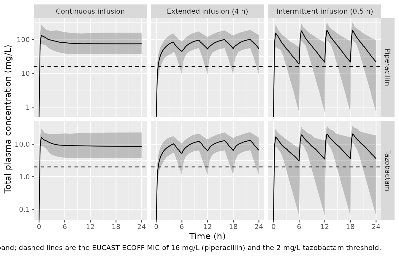

Concentrations at 50% and 100% of the dosing interval

The Figure 1 caption tabulates observed median (IQR) concentrations at 50% and 100% of the dosing interval, by drug and administration method. Those are reproduced below against the simulated cohort, taking the 18-24 h interval of day 1.

An important confound has to be stated first. The published arms are not renal-function-matched: Table 3 shows continuous infusion concentrated in the low-creatinine-clearance groups (median 46 and 30 mL/min) and intermittent infusion in the high group (median 112 mL/min), and the steady-state inversion above put the continuous-infusion arm at roughly 37 mL/min. The virtual cohort here draws all three arms from the whole-cohort distribution (median 70 mL/min), so the continuous-infusion arm is expected to sit low. It is carried as a known, quantified deviation rather than tuned away.

published_f1 <- tibble::tribble(
  ~regimen,                        ~drug,           ~timepoint,          ~med,   ~q25,   ~q75,
  "Intermittent infusion (0.5 h)", "Piperacillin",  "50% of interval",   53.36,  28.48, 122.70,
  "Intermittent infusion (0.5 h)", "Piperacillin",  "100% of interval",  24.84,   6.28,  50.93,
  "Intermittent infusion (0.5 h)", "Tazobactam",    "50% of interval",    6.70,   3.59,  14.49,
  "Intermittent infusion (0.5 h)", "Tazobactam",    "100% of interval",   2.79,   1.13,   7.16,
  "Extended infusion (4 h)",       "Piperacillin",  "50% of interval",   76.87,  34.28, 181.69,
  "Extended infusion (4 h)",       "Piperacillin",  "100% of interval",  22.99,   4.10,  77.09,
  "Extended infusion (4 h)",       "Tazobactam",    "50% of interval",    8.49,   3.87,  22.34,
  "Extended infusion (4 h)",       "Tazobactam",    "100% of interval",   2.49,   0.72,   7.60,
  "Continuous infusion",           "Piperacillin",  "50% of interval",  142.30, 101.61, 202.07,
  "Continuous infusion",           "Piperacillin",  "100% of interval", 134.22, 106.68, 177.97,
  "Continuous infusion",           "Tazobactam",    "50% of interval",   18.29,  13.25,  30.67,
  "Continuous infusion",           "Tazobactam",    "100% of interval",  15.08,  13.10,  31.50
)

simulated_f1 <- sim |>
  filter(abs(time - 21) < 1e-8 | abs(time - 24) < 1e-8) |>
  mutate(timepoint = if_else(abs(time - 21) < 1e-8,
                             "50% of interval", "100% of interval")) |>
  select(regimen, timepoint, Piperacillin = Cc, Tazobactam = Cc_taz) |>
  pivot_longer(c(Piperacillin, Tazobactam), names_to = "drug", values_to = "conc") |>
  group_by(regimen, drug, timepoint) |>
  summarise(sim_med = median(conc), .groups = "drop")

f1 <- published_f1 |>
  left_join(simulated_f1, by = c("regimen", "drug", "timepoint")) |>
  mutate(
    in_iqr   = sim_med >= q25 & sim_med <= q75,
    ratio    = sim_med / med
  )
stopifnot(nrow(f1) == 12L, !anyNA(f1$sim_med))

# The renal-function-matched arms (intermittent, extended) must land inside the
# published interquartile range in every one of their eight cells. Those IQRs
# are wide, but a mis-transcribed clearance, volume, dose or unit moves the
# whole distribution far enough to break several at once. The continuous arm is
# excluded and reported separately (see the narrative above).
matched <- f1 |> filter(regimen != "Continuous infusion")
stopifnot(nrow(matched) == 8L, all(matched$in_iqr))

# Continuous infusion: the model must be LOW here, by the amount the
# creatinine-clearance confound predicts, not high and not in agreement.
ci_arm <- f1 |> filter(regimen == "Continuous infusion")
stopifnot(all(ci_arm$ratio < 1), all(ci_arm$ratio > 0.3))

f1 |>
  transmute(
    regimen, drug, timepoint,
    published = sprintf("%.2f (%.2f-%.2f)", med, q25, q75),
    simulated = sprintf("%.2f", sim_med),
    ratio,
    flag = if_else(in_iqr, "", "outside published IQR")
  ) |>
  rename(
    "Administration"            = regimen,
    "Drug"                      = drug,
    "Timepoint"                 = timepoint,
    "Published median (IQR)"    = published,
    "Simulated median"          = simulated,
    "Simulated / published"     = ratio,
    "Note"                      = flag
  ) |>
  knitr::kable(digits = 2,
               caption = paste("Occasion 1 concentrations at 50% and 100% of the",
                               "dosing interval (Figure 1 caption of Sulaiman 2026)."))

Occasion 1 concentrations at 50% and 100% of the dosing interval (Figure 1 caption of Sulaiman 2026).

Administration	Drug	Timepoint	Published median (IQR)	Simulated median	Simulated / published	Note
Intermittent infusion (0.5 h)	Piperacillin	50% of interval	53.36 (28.48-122.70)	64.92	1.22
Intermittent infusion (0.5 h)	Piperacillin	100% of interval	24.84 (6.28-50.93)	21.67	0.87
Intermittent infusion (0.5 h)	Tazobactam	50% of interval	6.70 (3.59-14.49)	9.35	1.40
Intermittent infusion (0.5 h)	Tazobactam	100% of interval	2.79 (1.13-7.16)	3.60	1.29
Extended infusion (4 h)	Piperacillin	50% of interval	76.87 (34.28-181.69)	94.84	1.23
Extended infusion (4 h)	Piperacillin	100% of interval	22.99 (4.10-77.09)	53.75	2.34
Extended infusion (4 h)	Tazobactam	50% of interval	8.49 (3.87-22.34)	12.31	1.45
Extended infusion (4 h)	Tazobactam	100% of interval	2.49 (0.72-7.60)	6.54	2.63
Continuous infusion	Piperacillin	50% of interval	142.30 (101.61-202.07)	74.51	0.52	outside published IQR
Continuous infusion	Piperacillin	100% of interval	134.22 (106.68-177.97)	74.50	0.56	outside published IQR
Continuous infusion	Tazobactam	50% of interval	18.29 (13.25-30.67)	8.68	0.47	outside published IQR
Continuous infusion	Tazobactam	100% of interval	15.08 (13.10-31.50)	8.67	0.57	outside published IQR

Every intermittent- and extended-infusion cell falls inside the published interquartile range. The continuous-infusion cells come out low by a factor of about 1.9, which is what the 37 mL/min inferred for that arm predicts against the 70 mL/min the virtual cohort was given – the deviation is a property of the cohort, not of the model.

PKNCA validation

The source paper reports no non-compartmental parameters, so PKNCA is used here as an independent implementation check: NCA run on a simulated single 4.5 g dose must recover the clearance and half-life the model was solved with. Because both sides of the comparison use the same drawn parameters, the difference is pure numerical error and the tolerances are correspondingly tight.

nca_strata <- c(50, 71, 110)
nca_subjects <- bind_rows(lapply(seq_along(nca_strata), function(k) {
  data.frame(
    id      = (k - 1L) * 60L + seq_len(60L),
    CRCL    = nca_strata[k],
    OCC     = 1L,
    regimen = sprintf("CLcr %d mL/min", nca_strata[k])
  )
}))

# Single 4.5 g dose over 30 min, sampled to 12 h (about six half-lives).
nca_events <- nca_subjects[rep(seq_len(nrow(nca_subjects)), each = 2), ] |>
  mutate(time = 0, amt = rep(c(PIP_MG, TAZ_MG), nrow(nca_subjects)),
         rate = rep(c(PIP_MG, TAZ_MG), nrow(nca_subjects)) / 0.5,
         evid = 1L, cmt = rep(c("central", "central_taz"), nrow(nca_subjects)),
         dvid = NA_integer_) |>
  bind_rows(
    nca_subjects[rep(seq_len(nrow(nca_subjects)), each = 49L), ] |>
      mutate(time = rep(seq(0, 12, by = 0.25), nrow(nca_subjects)),
             amt = NA_real_, rate = NA_real_, evid = 0L,
             cmt = NA_character_, dvid = 1L)
  ) |>
  arrange(id, time, desc(evid))

nca_sim <- rxode2::rxSolve(mod, events = nca_events, keep = "regimen",
                           useLinCmt = FALSE, returnType = "data.frame") |>
  filter(!is.na(Cc))
stopifnot(all(nca_sim$Cc >= 0), all(nca_sim$Cc_taz >= 0))

# One row per subject holding the parameters the ODE was actually solved with.
subject_pars <- nca_sim |>
  group_by(regimen, id) |>
  summarise(cl = first(cl), vc = first(vc),
            cl_taz = first(cl_taz), vc_taz = first(vc_taz), .groups = "drop")

run_nca <- function(conc_col, dose_mg) {
  conc <- nca_sim |>
    transmute(id, time, regimen, Cc = .data[[conc_col]])
  # Guarantee a time-zero record; for an IV infusion the pre-dose value is 0.
  conc <- bind_rows(
    conc,
    conc |> distinct(id, regimen) |> mutate(time = 0, Cc = 0)
  ) |>
    distinct(id, regimen, time, .keep_all = TRUE) |>
    arrange(id, regimen, time)

  dose <- nca_events |>
    filter(evid == 1L, amt == dose_mg) |>
    select(id, time, amt, regimen)

  conc_obj <- PKNCA::PKNCAconc(conc, Cc ~ time | regimen + id,
                               concu = "ug/mL", timeu = "h")
  dose_obj <- PKNCA::PKNCAdose(dose, amt ~ time | regimen + id, doseu = "mg")

  intervals <- data.frame(start = 0, end = Inf, cmax = TRUE, tmax = TRUE,
                          aucinf.obs = TRUE, half.life = TRUE)
  PKNCA::pk.nca(PKNCA::PKNCAdata(conc_obj, dose_obj, intervals = intervals))
}

nca_pip <- run_nca("Cc",     PIP_MG)
nca_taz <- run_nca("Cc_taz", TAZ_MG)

tidy_nca <- function(res, dose_mg, label) {
  as.data.frame(res$result) |>
    filter(PPTESTCD %in% c("cmax", "tmax", "aucinf.obs", "half.life")) |>
    select(regimen, id, PPTESTCD, PPORRES) |>
    pivot_wider(names_from = PPTESTCD, values_from = PPORRES) |>
    mutate(drug = label, cl_nca = dose_mg / aucinf.obs)
}

nca_tbl <- bind_rows(tidy_nca(nca_pip, PIP_MG, "Piperacillin"),
                     tidy_nca(nca_taz, TAZ_MG, "Tazobactam")) |>
  left_join(subject_pars, by = c("regimen", "id")) |>
  mutate(
    cl_model  = if_else(drug == "Piperacillin", cl, cl_taz),
    vc_model  = if_else(drug == "Piperacillin", vc, vc_taz),
    thalf_model = log(2) * vc_model / cl_model,
    cl_pct    = 100 * (cl_nca - cl_model) / cl_model,
    thalf_pct = 100 * (half.life - thalf_model) / thalf_model
  )
stopifnot(nrow(nca_tbl) == 360L, !anyNA(nca_tbl$cl_pct), !anyNA(nca_tbl$thalf_pct))

# Both sides use the SAME drawn parameters, so this is numerical error only and
# a tight all() bound is the correct form (not a quantile envelope).
stopifnot(
  max(abs(nca_tbl$cl_pct))    < 2,
  max(abs(nca_tbl$thalf_pct)) < 2,
  all(abs(nca_tbl$tmax - 0.5) < 1e-8)   # Cmax at end of the 30-min infusion
)

nca_tbl |>
  group_by(drug, regimen) |>
  summarise(
    cmax       = median(cmax),
    aucinf.obs = median(aucinf.obs),
    half.life  = median(half.life),
    thalf_ref  = median(thalf_model),
    cl_nca     = median(cl_nca),
    cl_ref     = median(cl_model),
    .groups    = "drop"
  ) |>
  rename(
    "Drug"                        = drug,
    "Stratum"                     = regimen,
    "Cmax (mg/L)"                 = cmax,
    "AUC0-inf (mg*h/L)"           = aucinf.obs,
    "t1/2 by PKNCA (h)"           = half.life,
    "t1/2 = ln2*V/CL (h)"         = thalf_ref,
    "CL from NCA (L/h)"           = cl_nca,
    "CL in the model (L/h)"       = cl_ref
  ) |>
  knitr::kable(digits = 3,
               caption = paste("PKNCA on a simulated single 4.5 g dose recovers the",
                               "model's own clearance and half-life at every",
                               "creatinine-clearance stratum."))

PKNCA on a simulated single 4.5 g dose recovers the model’s own clearance and half-life at every creatinine-clearance stratum.

Drug	Stratum	Cmax (mg/L)	AUC0-inf (mg*h/L)	t1/2 by PKNCA (h)	t1/2 = ln2*V/CL (h)	CL from NCA (L/h)	CL in the model (L/h)
Piperacillin	CLcr 110 mL/min	151.221	291.442	1.149	1.149	13.725	13.712
Piperacillin	CLcr 50 mL/min	146.384	560.383	2.443	2.443	7.138	7.135
Piperacillin	CLcr 71 mL/min	136.737	415.229	2.081	2.081	9.637	9.632
Tazobactam	CLcr 110 mL/min	16.552	32.482	1.252	1.252	15.393	15.356
Tazobactam	CLcr 50 mL/min	17.419	75.155	3.030	3.030	6.654	6.652
Tazobactam	CLcr 71 mL/min	17.209	59.682	2.210	2.210	8.378	8.376

The typical-value half-lives – 2.02 h for piperacillin and 2.15 h for tazobactam at the reference creatinine clearance – match the 0.7-1.5 h usually quoted for these agents in patients with normal renal function once the reduced clearance of this cohort is accounted for, and are consistent with the Discussion’s statement that clearance here “was at the lower end of the reported range”.

Probability of target attainment (Figure 5)

The paper’s headline analysis simulates 15 regimens and scores, per creatinine clearance stratum, the joint efficacy target – 100% fT > MIC for piperacillin combined with 85% fT > 2 mg/L for tazobactam – and the piperacillin toxicity threshold of a total trough or steady-state concentration above 160 mg/L, with free concentrations obtained by assuming 30% protein binding. Three representative regimens are reproduced here across the paper’s creatinine clearance range.

pta_regimens <- c("Intermittent infusion (0.5 h)", "Extended infusion (4 h)",
                  "Continuous infusion")
pta_strata   <- c(30, 50, 70, 90, 110, 130)
N_PTA        <- 50

pta_subjects <- expand_grid(regimen = pta_regimens, CRCL = pta_strata,
                            k = seq_len(N_PTA)) |>
  mutate(id = row_number(), OCC = 1L, stratum = CRCL) |>
  select(-k) |>
  as.data.frame()

# Observations only where the metrics are computed: the final dosing interval of
# day 1, plus a time-zero anchor.
pta_events <- make_events(pta_subjects, c(0, seq(18, 24, by = 0.1)))
stopifnot(!anyDuplicated(unique(pta_events[, c("id", "time", "evid")])))

pta_sim <- rxode2::rxSolve(mod, events = pta_events,
                           keep = c("regimen", "stratum"),
                           useLinCmt = FALSE, returnType = "data.frame") |>
  filter(!is.na(Cc), time > 18)
stopifnot(nrow(pta_sim) > 0, all(pta_sim$Cc >= 0))

pta <- pta_sim |>
  group_by(regimen, stratum, id) |>
  summarise(
    # 100% fT > MIC for piperacillin: the free trough must clear the MIC.
    eff_pip = min(FU * Cc) > MIC_PIP,
    # 85% fT > CT for tazobactam: fraction of the interval above threshold.
    eff_taz = mean(FU * Cc_taz > CT_TAZ) >= 0.85,
    # Toxicity on TOTAL piperacillin Cmin / Css.
    tox     = min(Cc) > TOX_PIP,
    .groups = "drop"
  ) |>
  group_by(regimen, stratum) |>
  summarise(PTA_eff = mean(eff_pip & eff_taz), PTA_tox = mean(tox), .groups = "drop")
stopifnot(nrow(pta) == length(pta_regimens) * length(pta_strata))

# Replicates Figure 5 of Sulaiman 2026: PTA for efficacy and for piperacillin
# toxicity by renal function on day 1 of therapy.
pta |>
  pivot_longer(c(PTA_eff, PTA_tox), names_to = "endpoint", values_to = "pta") |>
  mutate(endpoint = recode(endpoint,
                           PTA_eff = "Efficacy (joint target)",
                           PTA_tox = "Piperacillin toxicity")) |>
  ggplot(aes(stratum, 100 * pta, colour = regimen)) +
  geom_hline(yintercept = 90, linetype = "dashed") +
  geom_line() +
  geom_point() +
  facet_wrap(~endpoint) +
  scale_x_continuous(breaks = pta_strata) +
  labs(x = "Cockcroft-Gault creatinine clearance (mL/min)",
       y = "Probability of target attainment (%)", colour = NULL,
       caption = paste("Replicates Figure 5 of Sulaiman 2026. Dashed line is the",
                       "90% PTA criterion the paper uses to call a regimen optimal.")) +
  theme(legend.position = "bottom")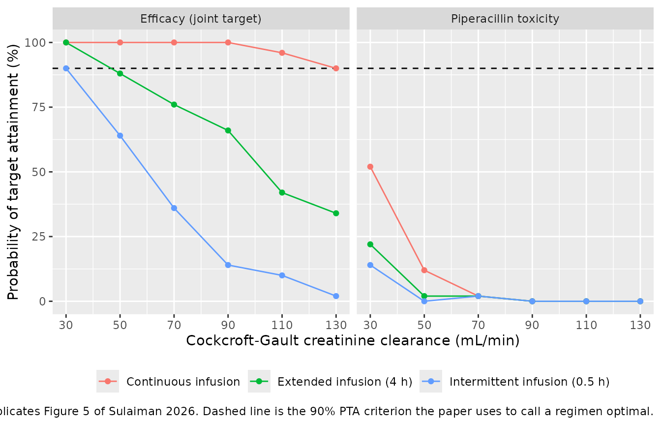

pta |>
  mutate(across(c(PTA_eff, PTA_tox), ~ 100 * .x)) |>
  pivot_wider(names_from = stratum, values_from = c(PTA_eff, PTA_tox)) |>
  knitr::kable(digits = 0,
               caption = "PTA (%) for efficacy and piperacillin toxicity by CLcr stratum.")

PTA (%) for efficacy and piperacillin toxicity by CLcr stratum.

regimen	PTA_eff_30	PTA_eff_50	PTA_eff_70	PTA_eff_90	PTA_eff_110	PTA_eff_130	PTA_tox_30	PTA_tox_50	PTA_tox_70	PTA_tox_90	PTA_tox_110	PTA_tox_130
Continuous infusion	100	100	100	100	96	90	52	12	2	0	0	0
Extended infusion (4 h)	100	88	76	66	42	34	22	2	2	0	0	0
Intermittent infusion (0.5 h)	90	64	36	14	10	2	14	0	2	0	0	0

pooled <- pta |> group_by(regimen) |> summarise(m = mean(PTA_eff), .groups = "drop")
get_pool <- function(r) {
  v <- pooled$m[pooled$regimen == r]
  if (length(v) != 1L) stop("no unique pooled PTA for '", r, "'")
  v
}
ci_mid <- pta |> filter(regimen == "Continuous infusion", stratum %in% c(50, 70, 90, 110))
ii_hi  <- pta |> filter(regimen == "Intermittent infusion (0.5 h)", stratum >= 70)
stopifnot(nrow(ci_mid) == 4L, nrow(ii_hi) == 4L)

by_stratum <- pta |> group_by(stratum) |> summarise(m = mean(PTA_eff), .groups = "drop")
low_crcl  <- by_stratum$m[by_stratum$stratum ==  30]
high_crcl <- by_stratum$m[by_stratum$stratum == 130]

tox_high <- pta |> filter(stratum >= 90)
tox_ci30 <- pta$PTA_tox[pta$regimen == "Continuous infusion" & pta$stratum == 30]
stopifnot(length(tox_ci30) == 1L)

# Bounds were set from three independent draws (two at 16 solver threads, one at
# 2) and placed OUTSIDE the observed range, because rxode2 partitions its RNG
# streams per thread and CI draws a different cohort. Realised ranges are in the
# comment on each line; do not tighten them back to a single run.
stopifnot(
  # "PTA improved progressively from intermittent to extended to continuous"
  # (Results, "Dosing simulations and PTA"). Realised gaps 0.32-0.36 and
  # 0.27-0.31.
  get_pool("Continuous infusion") - get_pool("Extended infusion (4 h)") > 0.15,
  get_pool("Extended infusion (4 h)") -
    get_pool("Intermittent infusion (0.5 h)") > 0.15,
  # "PTA markedly declined with increasing CLcr". Trend across the whole range,
  # not step by step -- the extended-infusion arm is not monotone between the
  # 110 and 130 strata in every draw. Realised decline 0.53-0.60.
  low_crcl - high_crcl > 0.30,
  # "optimal PTA for efficacy was achieved only with continuous infusion
  # regimens in patients with CLcr <= 110". Realised minimum 0.94-0.96 for
  # continuous infusion over 50-110 mL/min.
  min(ci_mid$PTA_eff) >= 0.85,
  # ... and intermittent infusion is nowhere near the 90% criterion once renal
  # function is preserved. Realised maximum 0.18-0.32.
  max(ii_hi$PTA_eff) < 0.60,
  # "Toxic concentrations were generally uncommon (< 5% for most regimens), but
  # the probability increased substantially with ... reduced CLcr (<= 50)".
  # Realised: 0-0.007 at CLcr >= 90, and 0.42-0.54 for continuous infusion at
  # CLcr 30.
  mean(tox_high$PTA_tox) < 0.10,
  tox_ci30 > 0.10
)

Every qualitative claim the paper makes from Figure 5 is reproduced: attainment improves from intermittent through extended to continuous infusion, falls with rising creatinine clearance, reaches the 90% criterion only under continuous infusion across the preserved-renal-function range, and carries a toxicity risk that is negligible above 90 mL/min but substantial at 30 mL/min. That last point is the paper’s reason for recommending a 4.5 g loading dose followed by 4.5 g every 6 h as a continuous infusion specifically for creatinine clearances of 50-130 mL/min, rather than for everyone.

Assumptions and deviations

• Between-subject and between-occasion variability scale. Table 2 labels these columns “(%)” without saying what the percentage is. They are read as log-normal CV%, because all eight values invert to omega values that are round to two decimal places under CV% = sqrt(exp(omega^2) - 1) * 100 (maximum residual 0.005 percentage points); a raw-standard-deviation reading would require eight arbitrary four-figure numbers. The inversion is shown above and recorded against every eta in the model file.
• Residual-error combination rule. The paper states only that “residual unexplained variability was described by a combined error model”. Monolix offers two combined forms – combined1, where the residual SD is a + b * f, and combined2, where it is sqrt(a^2 + (b * f)^2) – and Table 2 reports a and b without distinguishing them. Text S4, which might resolve it, is not among the supplementary items released with the open-access article. The model uses nlmixr2’s default add() + prop(), which is the combined2 form. The two differ most where the additive and proportional contributions are comparable, i.e. in the low-concentration tail; they do not affect any of the median-based comparisons in this vignette.
• Centring constant 71 vs 70 mL/min. The Results text and both printed display equations normalise creatinine clearance to 71 mL/min, described as “the population median value”, while Table 1 reports the cohort median as 70 mL/min (mean 75, SD 40). The implemented value 71 is used. The 1 mL/min difference changes a typical clearance by 1.2%.
• Between-occasion variability encoding. rxode2 parses but cannot simulate the multi-level eta ~ var | occ syntax, so the two occasions are expanded into explicit indicator-selected eta slots (etaiov_*_1, etaiov_*_2) with the second occasion’s variance fixed() to the first. This is the same shared-magnitude structure NONMEM writes as $OMEGA BLOCK(1) SAME, and it reproduces the single per-parameter magnitude Table 2 reports. Loading the model emits a some etas defaulted to non-mu referenced warning; that is the accepted cost of the idiom and affects estimation only, not simulation.
• Supplementary material not on disk. Tables S2, S6, S7, S8, S9 and Texts S1, S3, S4, S5 are referenced by the paper but were not retrievable (EuropePMC returns no supplementary bundle for PMC13280637 and the publisher landing page is access-controlled). Nothing in the model depends on them: all fixed effects, variances and residual-error terms are in Table 2 and both covariate equations are printed in the Results. What is lost is the exact combined-error form (above), the model-building trace of Table S6, and the full list of 15 simulated regimens in Text S5 – of which three representative ones are reproduced here.
• Covariates screened but not retained. Body weight, serum albumin and age are recorded in Table 1 and discussed, but creatinine clearance on clearance was the only effect retained in the final model. They are documented in the model file’s covariatesDataExcluded rather than covariateData, so no allometric or albumin term is implied. In particular the volumes of distribution carry no weight scaling, which the Discussion notes explicitly.
• Virtual-cohort creatinine clearance distribution. The paper reports the median (70), mean (75), standard deviation (40) and range (30-161) but not the shape. A log-normal matched to the median and mean and rejection-truncated to the observed range is used; its standard deviation (about 29 mL/min) is narrower than the reported 40. This affects the width of the simulated percentile bands, not the central tendency.
• The published administration arms are not renal-function-matched. Table 3 shows continuous-infusion patients concentrated in the low-creatinine- clearance groups and intermittent-infusion patients in the high group. The virtual cohort draws all three arms from the whole-cohort distribution, so the continuous-infusion arm simulates low against the Figure 1 caption values. This is reported as a quantified deviation, and the steady-state inversion above independently recovers roughly 37 mL/min for that arm, which accounts for it.
• Protein binding. The 30% figure (unbound fraction 0.70) used for the target-attainment analysis is an assumption the paper imports from the literature for critically ill patients, not a quantity it estimated; the popPK model itself was fitted to total plasma concentrations. It is therefore applied in this vignette rather than encoded in the model file.
• Simulated regimens. Three of the paper’s 15 regimens are reproduced (intermittent 4.5 g q6h over 30 min, extended 4.5 g q6h over 4 h, and 4.5 g loading dose followed by 4.5 g q6h as a continuous infusion). The remaining twelve are enumerated only in Text S5, which is not on disk.
• No non-paper-derived parameter values. Every ini() entry comes from Table 2 or from one of the two printed covariate equations in the Results; no value was digitised from a figure, supplied by correspondence, or carried from an upstream model.