Fentanyl PBPK and its proper-lumped reductions (Pan 2019)

Model and source

Pan and Duffull (2019) automate proper lumping (Dokoumetzidis and Aarons): a linear ODE system dC/dt = K C is reduced to dC_hat/dt = K_hat C_hat with K_hat = M K M+ (their Eq. 2), where M is a 0/1 lumping matrix and M+ its Moore-Penrose pseudo-inverse. The worked example is the 16-state whole-body fentanyl PBPK model of Bjorkman et al. (1994), which they reduce to two different 4-state models (Figure 4a and 4b) with arterial blood held unlumped as the observed state. All three structures ship in nlmixr2lib:

Model	States	Source
Pan_2019_fentanyl_pbpk	16 (original PBPK)	Supplementary Material 1 Sections 1A-1B; deposited Model_parameter_values.m
Pan_2019_fentanyl_lumped_a	venous, arterial, lumped1, lumped2	Figure 4a; Supplementary Section 2
Pan_2019_fentanyl_lumped_b	lumped1, arterial, lumped2, lumped3	Figure 4b; Supplementary Section 3

• Citation: Pan S, Duffull SB (2019). Automated proper lumping for simplification of linear physiologically based pharmacokinetic systems. J Pharmacokinet Pharmacodyn 46(4):361-370. doi:10.1007/s10928-019-09644-5. Parameter values and the 16 x 16 micro-rate-constant matrix from Supplementary Material 1 Sections 1A-1B and the deposited MATLAB files (Model_parameter_values.m, Runfile_Autolumping_FenPBPK.m). Physiology originally from Bjorkman S, Stanski DR, Verotta D, Harashima H (1994) Comparative tissue concentration profiles of fentanyl and alfentanil in humans predicted from tissue/blood partition data obtained in rats. Anesthesiology 80:380-393 (cited as ref 15).
• Article: https://doi.org/10.1007/s10928-019-09644-5 (open access)
• Full text, Supplementary Material 1 and the deposited MATLAB code: https://europepmc.org/article/PMC/PMC6656793

mod_names <- c(
  full = "Pan_2019_fentanyl_pbpk",
  a = "Pan_2019_fentanyl_lumped_a",
  b = "Pan_2019_fentanyl_lumped_b"
)
ui <- lapply(mod_names, function(n) rxode2::rxode(readModelDb(n)))

Population

There is no fitted cohort. The model describes one deterministic 73 kg reference man (Supplementary Section 1A, WT = 73; % average weight for man) with a cardiac output of 6.7 L/min. Organ volumes, blood flows and tissue:blood partition coefficients are those Bjorkman et al. (1994) scaled to man from rat tissue/blood partition data. Pan 2019 simulate a single 750 ug intravenous bolus and observe arterial blood over 0-210 min (deposited Runfile_Autolumping_FenPBPK.m). No between-subject variability or residual error is defined anywhere in the paper.

str(ui$full$population)
#> List of 7
#>  $ species      : chr "human"
#>  $ n_subjects   : int 1
#>  $ age_range    : chr "adult (reference man)"
#>  $ weight_range : chr "73 kg (reference man)"
#>  $ disease_state: chr "Not applicable: a physiology-based reference individual, not a fitted cohort."
#>  $ dose_range   : chr "750 ug intravenous bolus (Pan 2019); 750 ug over 5 min in the original Bjorkman 1994 study"
#>  $ notes        : chr "A single deterministic reference individual: Supplementary Material 1 Section 1A gives WT = 73 kg ('average wei"| __truncated__

Source trace

Every ini() value carries an in-file comment pointing to its source line. In summary:

Equation / parameter	Value	Source location
qc	6.7 L/min	Suppl. 1A Qcad = 6.7
v_venous, v_arterial	3.9, 2.0 L	Suppl. 1A Vven, Vart
v_<organ> (brain, heart, kidney, liver, muscle, skin, adipose, other = carcass, gut)	1.4, 0.33, 0.31, 1.8, 30, 3.3, 12.5, 15.5, 1.2 L	Suppl. 1A V<org>
qn_<organ> (blood flow per kg tissue)	0.56, 0.8, 4, 0.96, 0.038, 0.12, 0.028, 0.04, 0.83 L/min/kg	Suppl. 1A Q<org> = <x>*V<org>
lkp_<organ>	log(4), log(5.1), log(13.7), log(4.3), log(3.5), log(2.3), log(30.3), log(1), log(9)	Suppl. 1A KP<org>; carcass “not available”, set to 1
v_spleen, qn_spleen, lkp_spleen (pancreas + spleen)	0.14 L, 0.9 L/min/kg, log(27.7)	Suppl. 1A Vpas = (0.18+0.10)/2, Qpas = (0.6+1.2)/2*Vpas, KPpas = (24.1+31.3)/2
cln_spleen_deep, vn_spleen, vn_spleen_deep	2.21 L/min/kg, 0.082, 22.3 L/kg	Suppl. 1A CL12_pas, Vpas_1, Vpas_2 (Bjorkman p 388)
cln_liver_deep, cln_liver, vn_liver_deep	0.35, 0.095 L/min/kg, 8.7 L/kg	Suppl. 1A CL12_hep, CL10_hep, Vhep_2
cln_gut_deep, cln_gut_deep2, vn_gut_deep, vn_gut_deep2	0.89, 0.03 L/min/kg, 6.4, 3.26 L/kg	Suppl. 1A CL12_gut, CL23_gut, Vgut_2, Vgut_3
ODE system of Pan_2019_fentanyl_pbpk	rows 1-16 of K	Suppl. 1B; Model_parameter_values.m state equations
Dose into venous as Dose / Vven	f(venous) <- 1 / v_venous	Runfile IC = [Dose/Vven; zeros(15,1)]
Observation Cc <- arterial	state 2	Runfile output = [2]
Lumping matrices M	Figure 4a / 4b membership	Figure 4
Lumped rate constants k_<from>_<to>, kloss_<state>	K_hat = M K M+	Eq. 2; printed to 2 decimals in Suppl. Sections 2 and 3

Original 16-state system against the deposited matrix

The model file writes the 16 ODEs term by term. As an independent check, the matrix K of Supplementary Section 1B is rebuilt here from the model’s own ini() values and solved with the eigen-decomposition matrix exponential the authors use (ME_solution_function.m). Both sides use identical parameters, so the only difference is ODE integration error and a tight bound is appropriate.

build_k <- function(th) {
  p <- as.list(th)
  kp <- function(o) exp(p[[paste0("lkp_", o)]])
  q <- function(o) p[[paste0("qn_", o)]] * p[[paste0("v_", o)]]
  kt <- function(o) q(o) / (p[[paste0("v_", o)]] * kp(o))
  st <- c(
    "venous", "arterial", "brain", "heart", "kidney", "liver", "muscle",
    "skin", "adipose", "other", "gut", "gut_deep", "gut_deep2", "spleen",
    "spleen_deep", "liver_deep"
  )
  k <- matrix(0, 16, 16, dimnames = list(st, st))
  perf <- c("brain", "heart", "kidney", "liver", "muscle", "skin", "adipose", "other")
  k["venous", "venous"] <- -p$qc / p$v_venous
  for (o in perf) k["venous", o] <- kt(o) * p[[paste0("v_", o)]] / p$v_venous
  k["arterial", "venous"] <- p$qc / p$v_arterial
  k["arterial", "arterial"] <- -p$qc / p$v_arterial
  for (o in setdiff(perf, "liver")) {
    k[o, "arterial"] <- q(o) / p[[paste0("v_", o)]]
    k[o, o] <- -kt(o)
  }
  v_liv <- p$v_liver
  cl12_hep <- p$cln_liver_deep * v_liv
  cl10_hep <- p$cln_liver * v_liv
  v_hep2 <- p$vn_liver_deep * v_liv
  k["liver", "liver"] <- -(cl12_hep + cl10_hep) / v_liv - kt("liver")
  k["liver", "gut"] <- kt("gut") * p$v_gut / v_liv
  k["liver", "spleen"] <- kt("spleen") * p$v_spleen / v_liv
  k["liver", "liver_deep"] <- cl12_hep / v_liv
  cl12_gut <- p$cln_gut_deep * p$v_gut
  cl23_gut <- p$cln_gut_deep2 * p$v_gut
  v_gut2 <- p$vn_gut_deep * p$v_gut
  v_gut3 <- p$vn_gut_deep2 * p$v_gut
  k["gut", "arterial"] <- q("gut") / p$v_gut
  k["gut", "gut"] <- -(q("gut") + cl12_gut) / p$v_gut
  k["gut", "gut_deep"] <- cl12_gut / p$v_gut
  k["gut_deep", "gut"] <- cl12_gut / v_gut2
  k["gut_deep", "gut_deep"] <- -(cl12_gut + cl23_gut) / v_gut2
  k["gut_deep", "gut_deep2"] <- cl23_gut / v_gut2
  k["gut_deep2", "gut_deep"] <- cl23_gut / v_gut3
  k["gut_deep2", "gut_deep2"] <- -cl23_gut / v_gut3
  cl12_pas <- p$cln_spleen_deep * p$v_spleen
  v_pas1 <- p$vn_spleen * p$v_spleen
  v_pas2 <- p$vn_spleen_deep * p$v_spleen
  k["spleen", "arterial"] <- q("spleen") / v_pas1
  k["spleen", "spleen"] <- -(q("spleen") + cl12_pas) / v_pas1
  k["spleen", "spleen_deep"] <- cl12_pas / v_pas1
  k["spleen_deep", "spleen"] <- cl12_pas / v_pas2
  k["spleen_deep", "spleen_deep"] <- -cl12_pas / v_pas2
  k["liver_deep", "liver"] <- cl12_hep / v_hep2
  k["liver_deep", "liver_deep"] <- -cl12_hep / v_hep2
  k
}

# Matrix-exponential solution, as in the authors' ME_solution_function.m.
me_solution <- function(k, ic, times) {
  e <- eigen(k)
  q <- solve(e$vectors, ic)
  Re(e$vectors %*% (q * exp(outer(e$values, times))))
}

K <- build_k(ui$full$theta)
dose <- 750
ic_full <- c(dose / ui$full$theta[["v_venous"]], rep(0, 15))
times_runfile <- seq(0, 210, by = 0.5)

ev_full <- rxode2::et(amt = dose, cmt = "venous", time = 0) |>
  rxode2::et(times_runfile)
sim_full <- as.data.frame(
  rxode2::rxSolve(ui$full, ev_full, rtol = 1e-10, atol = 1e-12)
)
cf_full <- me_solution(K, ic_full, times_runfile)
rel_err <- abs(sim_full$arterial[-1] / cf_full[2, -1] - 1)
max(rel_err)
#> [1] 2.064671e-10
# ODE vs closed form on identical parameters; measured ~1e-10 at these
# tolerances.
stopifnot(max(rel_err) < 1e-7)

Lumped rate matrices (Eq. 2) against Supplementary Sections 2 and 3

The lumping matrices are read off Figure 4. Applying Eq. 2 to the rebuilt K reproduces both printed matrices entry for entry at the printed precision. Supplementary Section 3 orders the two tissue lumps of model b as L3 then L2 (the arterial inflow column, 0.60 = 0.56 + 0.038 for brain plus muscle, identifies L3), so its rows and columns are reordered here before comparison.

make_m <- function(groups, states = rownames(K)) {
  m <- matrix(0, length(groups), length(states), dimnames = list(names(groups), states))
  for (g in names(groups)) m[g, groups[[g]]] <- 1
  m
}
# Moore-Penrose pseudo-inverse of a full-row-rank 0/1 lumping matrix.
pinv_m <- function(m) t(m) %*% solve(m %*% t(m))
lump_k <- function(m) m %*% K %*% pinv_m(m)

m_a <- make_m(list(
  venous = "venous", arterial = "arterial",
  lumped1 = c(
    "brain", "heart", "kidney", "liver", "skin", "gut", "gut_deep",
    "gut_deep2", "spleen", "spleen_deep", "liver_deep"
  ),
  lumped2 = c("muscle", "adipose", "other")
))
m_b <- make_m(list(
  lumped1 = c("venous", "other", "gut", "gut_deep"), arterial = "arterial",
  lumped2 = c("heart", "kidney", "spleen", "skin", "adipose", "liver", "liver_deep"),
  lumped3 = c("brain", "muscle", "gut_deep2", "spleen_deep")
))
khat_a <- lump_k(m_a)
khat_b <- lump_k(m_b)

printed_a <- matrix(
  c(
    -1.72, 0, 0.02, 0.08,
    3.35, -3.35, 0, 0,
    0, 17.3, -1.15, 0,
    0, 0.11, 0, -0.02
  ),
  4, byrow = TRUE
)
# Supplement order L1, arterial, L3, L2; reorder to lumped1, arterial,
# lumped2 (= L2), lumped3 (= L3).
printed_b_suppl <- matrix(
  c(
    -0.61, 0.87, 0.03, 0.03,
    0.84, -3.35, 0, 0,
    0.002, 0.60, -0.06, 0.01,
    0.02, 15.9, 6.74, -5.53
  ),
  4, byrow = TRUE
)
ord <- c(1, 2, 4, 3)
printed_b <- printed_b_suppl[ord, ord]

# Each printed entry has its own number of decimals (17.3, -1.15, 0.002), so
# compare each at half a unit in its own last printed place. Printed zeros are
# structural and must be exactly zero.
printed_decimals <- function(x) {
  vapply(x, function(v) nchar(sub("^[0-9]*\\.?", "", sub("0+$", "", sprintf("%.6f", abs(v))))), 1)
}
matches_print <- function(computed, printed) {
  tol <- 0.5 * 10^-printed_decimals(printed)
  nz <- printed != 0
  all(abs(computed[nz] - printed[nz]) <= tol[nz] + 1e-12) && all(computed[!nz] == 0)
}
round(khat_a, 4)
#>           venous arterial lumped1 lumped2
#> venous   -1.7179   0.0000  0.0213  0.0818
#> arterial  3.3500  -3.3500  0.0000  0.0000
#> lumped1   0.0000  17.2856 -1.1546  0.0000
#> lumped2   0.0000   0.1060  0.0000 -0.0173
round(khat_b, 4)
#>          lumped1 arterial lumped2 lumped3
#> lumped1  -0.6084   0.8700  0.0267  0.0346
#> arterial  0.8375  -3.3500  0.0000  0.0000
#> lumped2   0.0154  15.9236 -5.5349  6.7378
#> lumped3   0.0023   0.5980  0.0142 -0.0648
stopifnot(matches_print(khat_a, printed_a), matches_print(khat_b, printed_b))

The packaged lumped models carry these Eq. 2 values unrounded (to six significant figures). The check below rebuilds each model’s rate matrix from its ini() and compares it with K_hat.

khat_from_ini <- function(th, states) {
  k <- matrix(0, length(states), length(states), dimnames = list(states, states))
  for (nm in names(th)) {
    if (startsWith(nm, "kloss_")) {
      s <- sub("^kloss_", "", nm)
      k[s, s] <- -th[[nm]]
    } else if (startsWith(nm, "k_")) {
      ft <- strsplit(sub("^k_", "", nm), "_")[[1]]
      k[ft[2], ft[1]] <- th[[nm]]
    }
  }
  k
}
ini_a <- khat_from_ini(ui$a$theta, rownames(khat_a))
ini_b <- khat_from_ini(ui$b$theta, rownames(khat_b))
max(abs(ini_a - khat_a) / pmax(abs(khat_a), 1e-12))
#> [1] 3.501637e-06
max(abs(ini_b - khat_b) / pmax(abs(khat_b), 1e-12))
#> [1] 1.927711e-06
# Six significant figures in ini(): relative rounding <= 5e-6.
stopifnot(
  all(abs(ini_a - khat_a) <= 1e-5 * abs(khat_a)),
  all(abs(ini_b - khat_b) <= 1e-5 * abs(khat_b))
)

Replicate Figure 6: arterial profiles of the original and lumped models

Pan 2019 Figure 6 overlays the arterial profile of each lumped model on the original over 0-360 min. The packaged models are simulated below. The dotted lines repeat each lumped simulation with the rate constants rounded to the two decimals printed in the supplement.

times_fig <- sort(unique(c(seq(0, 2, by = 0.05), seq(2, 360, by = 1))))
sim_cc <- function(u, cmt, params = NULL) {
  ev <- rxode2::et(amt = dose, cmt = cmt, time = 0) |> rxode2::et(times_fig)
  out <- if (is.null(params)) {
    rxode2::rxSolve(u, ev, rtol = 1e-10, atol = 1e-12)
  } else {
    rxode2::rxSolve(u, ev, params = params, rtol = 1e-10, atol = 1e-12)
  }
  as.data.frame(out)[, c("time", "Cc")]
}
printed_params <- function(u, printed, states) {
  th <- u$theta
  for (nm in names(th)) {
    if (startsWith(nm, "kloss_")) {
      s <- sub("^kloss_", "", nm)
      th[[nm]] <- -printed[match(s, states), match(s, states)]
    } else if (startsWith(nm, "k_")) {
      ft <- strsplit(sub("^k_", "", nm), "_")[[1]]
      th[[nm]] <- printed[match(ft[2], states), match(ft[1], states)]
    }
  }
  th
}

fig6 <- bind_rows(
  sim_cc(ui$full, "venous") |> mutate(model = "Original model", panel = "a"),
  sim_cc(ui$full, "venous") |> mutate(model = "Original model", panel = "b"),
  sim_cc(ui$a, "venous") |> mutate(model = "Lumped (Eq. 2)", panel = "a"),
  sim_cc(ui$b, "lumped1") |> mutate(model = "Lumped (Eq. 2)", panel = "b"),
  sim_cc(ui$a, "venous", printed_params(ui$a, printed_a, rownames(khat_a))) |>
    mutate(model = "Lumped (printed 2 dp)", panel = "a"),
  sim_cc(ui$b, "lumped1", printed_params(ui$b, printed_b, rownames(khat_b))) |>
    mutate(model = "Lumped (printed 2 dp)", panel = "b")
) |>
  mutate(panel = paste("Lumped model", panel))

ggplot(filter(fig6, time > 0), aes(time, Cc, colour = model, linetype = model)) +
  geom_line() +
  facet_wrap(~panel) +
  scale_y_log10(limits = c(1e-2, 1e2)) +
  scale_colour_manual(values = c("Original model" = "blue", "Lumped (Eq. 2)" = "red", "Lumped (printed 2 dp)" = "grey40")) +
  scale_linetype_manual(values = c("Original model" = "solid", "Lumped (Eq. 2)" = "dashed", "Lumped (printed 2 dp)" = "dotted")) +
  labs(x = "Time (min)", y = "Arterial concentration (ug/L)", colour = NULL, linetype = NULL) +
  theme_bw() +
  theme(legend.position = "bottom")
#> Warning: Removed 55 rows containing missing values or values outside the scale range
#> (`geom_line()`).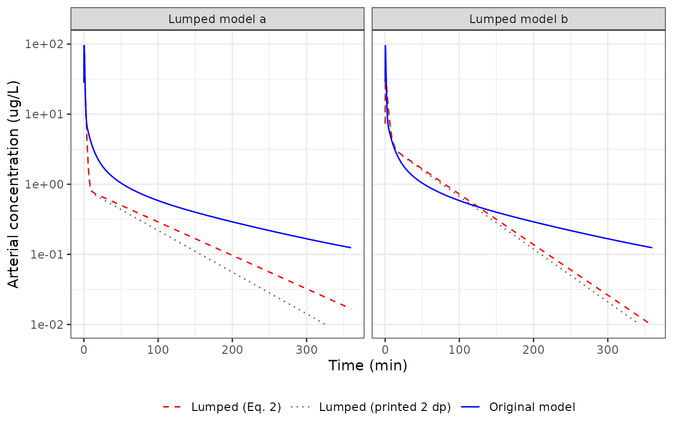

Replicates Figure 6 of Pan 2019. Values read off the published figure at 360 min are about 0.13 ug/L for the original model, 0.018 ug/L for lumped model a and 0.01 ug/L for lumped model b; lumped model b crosses the original at about 120 min, and lumped model a sits near 0.75 ug/L at 15 min. The Eq. 2 rate constants reproduce all of these. The two-decimal print of the supplement does not hold the terminal phase of model a, because its slowest constant (0.0173/min) prints as 0.02/min.

at <- function(m, p, t) {
  d <- filter(fig6, model == m, panel == p)
  approx(d$time, d$Cc, xout = t)$y
}
fig6_points <- tibble::tribble(
  ~quantity, ~figure, ~simulated,
  "Original, 360 min", 0.13, at("Original model", "Lumped model a", 360),
  "Lumped a, 15 min", 0.75, at("Lumped (Eq. 2)", "Lumped model a", 15),
  "Lumped a, 360 min", 0.018, at("Lumped (Eq. 2)", "Lumped model a", 360),
  "Lumped b, 360 min", 0.01, at("Lumped (Eq. 2)", "Lumped model b", 360),
  "Lumped a (printed 2 dp), 360 min", 0.018, at("Lumped (printed 2 dp)", "Lumped model a", 360)
)
knitr::kable(fig6_points, digits = 4)

quantity	figure	simulated
Original, 360 min	0.130	0.1243
Lumped a, 15 min	0.750	0.7386
Lumped a, 360 min	0.018	0.0167
Lumped b, 360 min	0.010	0.0097
Lumped a (printed 2 dp), 360 min	0.018	0.0062

d_b <- filter(fig6, panel == "Lumped model b", model != "Lumped (printed 2 dp)") |>
  select(time, model, Cc) |>
  pivot_wider(names_from = model, values_from = Cc) |>
  filter(time >= 30)
t_cross <- d_b$time[which(d_b[["Lumped (Eq. 2)"]] < d_b[["Original model"]])[1]]
t_cross
#> [1] 126

# Deterministic simulation against values read off a log-scale figure: a
# 20% band covers reading error, while a wrong rate constant or lumping
# assignment moves the 360 min value by several-fold.
stopifnot(
  all(abs(fig6_points$simulated[1:4] / fig6_points$figure[1:4] - 1) < 0.2),
  t_cross > 100, t_cross < 140
)

Replicate Figure 7: lumped tissue against its member tissues

A lumped state is the sum of the concentrations of the original states it pools (C_hat = M C). Figure 7 plots the third lumped state (L3) of each model against its member tissues in the original model.

ev_fig <- rxode2::et(amt = dose, cmt = "venous", time = 0) |> rxode2::et(times_fig)
full_tis <- as.data.frame(rxode2::rxSolve(ui$full, ev_fig, rtol = 1e-10, atol = 1e-12))
lump_a <- as.data.frame(rxode2::rxSolve(ui$a, ev_fig, rtol = 1e-10, atol = 1e-12))
ev_b <- rxode2::et(amt = dose, cmt = "lumped1", time = 0) |> rxode2::et(times_fig)
lump_b <- as.data.frame(rxode2::rxSolve(ui$b, ev_b, rtol = 1e-10, atol = 1e-12))

fig7 <- bind_rows(
  full_tis |>
    select(time, muscle, adipose, other) |>
    pivot_longer(-time, names_to = "state", values_to = "conc") |>
    mutate(panel = "Model a: L3 = muscle, adipose, carcass"),
  lump_a |>
    transmute(time, state = "lumped2 (L3)", conc = lumped2, panel = "Model a: L3 = muscle, adipose, carcass"),
  full_tis |>
    select(time, brain, muscle, gut_deep2, spleen_deep) |>
    pivot_longer(-time, names_to = "state", values_to = "conc") |>
    mutate(panel = "Model b: L3 = brain, muscle, gut_deep2, spleen_deep"),
  lump_b |>
    transmute(time, state = "lumped3 (L3)", conc = lumped3, panel = "Model b: L3 = brain, muscle, gut_deep2, spleen_deep")
)

ggplot(filter(fig7, time > 0), aes(time, conc, colour = state, linetype = grepl("^lumped", state))) +
  geom_line() +
  facet_wrap(~panel) +
  scale_y_log10(limits = c(1e-2, 1e3)) +
  scale_linetype_manual(values = c(`FALSE` = "solid", `TRUE` = "dashed"), guide = "none") +
  labs(x = "Time (min)", y = "Tissue concentration (ug/L)", colour = NULL) +
  theme_bw() +
  theme(legend.position = "bottom")
#> Warning: Removed 22 rows containing missing values or values outside the scale range
#> (`geom_line()`).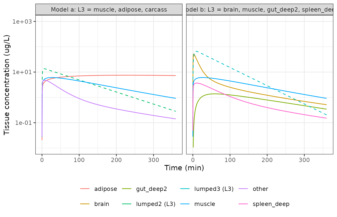

Replicates Figure 7 of Pan 2019 (lumped model a peaks near 13 ug/L, lumped model b near 70 ug/L).

peak_a <- max(lump_a$lumped2)
peak_b <- max(lump_b$lumped3)
c(peak_a = peak_a, peak_b = peak_b)
#>   peak_a   peak_b 
#> 13.56888 65.76847
# Read off the log-scale figure; a 25% band covers reading error.
stopifnot(abs(peak_a / 13 - 1) < 0.25, abs(peak_b / 70 - 1) < 0.25)

NCA of the arterial profile (PKNCA)

The paper’s acceptance criterion is the absolute relative difference (ARD%) in arterial AUC over the runfile grid, 0-210 min in 0.5 min steps, computed with the linear trapezoidal rule (cumtrapz). The NCA below uses the same grid and the linear rule.

sim_runfile <- function(u, cmt, label) {
  ev <- rxode2::et(amt = dose, cmt = cmt, time = 0) |> rxode2::et(times_runfile)
  out <- as.data.frame(rxode2::rxSolve(u, ev, rtol = 1e-10, atol = 1e-12))
  # A single-subject solve returns no id column.
  out$id <- 1L
  out$model <- label
  out[, c("id", "model", "time", "Cc")]
}
nca_conc <- bind_rows(
  sim_runfile(ui$full, "venous", "Original (16 states)"),
  sim_runfile(ui$a, "venous", "Lumped a (4 states)"),
  sim_runfile(ui$b, "lumped1", "Lumped b (4 states)")
) |>
  filter(!is.na(Cc))
nca_dose <- distinct(nca_conc, id, model) |> mutate(time = 0, amt = dose)

conc_obj <- PKNCA::PKNCAconc(nca_conc, Cc ~ time | model + id)
dose_obj <- PKNCA::PKNCAdose(nca_dose, amt ~ time | model + id)
intervals <- data.frame(
  start = 0, end = 210, cmax = TRUE, tmax = TRUE, auclast = TRUE,
  aucinf.obs = TRUE, half.life = TRUE
)
nca_res <- PKNCA::pk.nca(
  PKNCA::PKNCAdata(conc_obj, dose_obj,
    intervals = intervals,
    options = list(auc.method = "linear")
  )
)
nca_tab <- as.data.frame(nca_res) |>
  filter(PPTESTCD %in% c("cmax", "tmax", "auclast", "aucinf.obs", "half.life")) |>
  select(model, PPTESTCD, PPORRES) |>
  pivot_wider(names_from = PPTESTCD, values_from = PPORRES)
auc_full <- nca_tab$auclast[nca_tab$model == "Original (16 states)"]
nca_tab <- nca_tab |>
  mutate(ard_pct = 100 * abs(auclast - auc_full) / auc_full) |>
  select(model, cmax, tmax, auclast, ard_pct, aucinf.obs, half.life)
nca_tab |>
  rename(
    "Model" = model,
    "Cmax (ug/L)" = cmax,
    "Tmax (min)" = tmax,
    "AUC0-210 (ug min/L)" = auclast,
    "ARD% in AUC0-210 vs original" = ard_pct,
    "AUC0-inf (ug min/L)" = aucinf.obs,
    "t1/2 (min)" = half.life
  ) |>
  knitr::kable(digits = 3)

Model	Cmax (ug/L)	Tmax (min)	AUC0-210 (ug min/L)	ARD% in AUC0-210 vs original	AUC0-inf (ug min/L)	t1/2 (min)
Lumped a (4 states)	93.970	0.5	194.083	35.804	201.967	63.047
Lumped b (4 states)	33.547	1.0	325.628	7.707	332.644	41.658
Original (16 states)	93.574	0.5	302.329	0.000	347.375	113.811

# The trapezoidal AUC of the original model equals the closed-form solution
# integrated on the same grid (same parameters, so a tight bound).
auc_cf <- sum(diff(times_runfile) * (head(cf_full[2, ], -1) + tail(cf_full[2, ], -1)) / 2)
stopifnot(abs(auc_full / auc_cf - 1) < 1e-6)
# Deterministic: pins the ARD% values quoted in the text below.
ard <- setNames(nca_tab$ard_pct, nca_tab$model)
stopifnot(
  abs(ard[["Lumped a (4 states)"]] - 36) < 1,
  abs(ard[["Lumped b (4 states)"]] - 8) < 1
)

The paper does not report Cmax, Tmax, AUC or half-life for any of the three models, so there is no published NCA table to compare against. What it does report – an ARD% of at most 0.002% for every accepted 4-state model – is not reproduced: on the authors’ own grid and rule the ARD% is about 36% for lumped model a and about 8% for lumped model b. See the Errata below.

Assumptions and deviations

• Dosing site: venous, not arterial. The Methods say “an arterial bolus was used” and the Discussion “a single bolus dose into the arterial blood compartment”, but the deposited runfile sets IC = [Dose/Vven; zeros(15,1)], i.e. the bolus enters state 1 (venous) as Dose / Vven. The deposited code is the executable source of the published matrices and figures, so it is followed: each model doses into venous (model b: into the venous-containing lumped1) with f() <- 1 / v_venous, so that a dose record of 750 ug reproduces the paper’s initial condition.
• 16 states, not 17. The paper says “In total there were 17 states” and Figure 4a labels the venous state “Venous blood, Lung”, but the deposited K is 16 x 16 and sets the lung concentration equal to the venous concentration (% Clun = Cven). The lung parameters of Section 1A (Vlun, Qlun, KPlun) are computed and never used, so they are not carried in ini().
• The deposited K is not flow-conserving. The liver receives no arterial inflow in K (only portal inflow from gut and pancreas + spleen), and the gut and pancreas + spleen first compartments lose drug at Q * C but deliver Q * C / KP to the liver. Arterial outflow to the tissues sums to 6.04 L/min against a cardiac output of 6.7 L/min. These are properties of the authors’ matrix, which is transcribed unchanged; they are not corrected here.
• Pancreas + spleen as spleen. Bjorkman’s pancreas and spleen are averaged into one tissue (Vpas, Qpas, KPpas are means of the two), which Figure 4 labels “Spleen”. The canonical spleen / spleen_deep names are used with the pooling stated in the model description. Carcass is the canonical other; fat is the canonical adipose.
• Lumped rate constants from Eq. 2, not the two-decimal print. The supplement prints K_hat to two decimals. Each packaged value is the Eq. 2 result from the sourced K and the Figure 4 lumping, and every one rounds to the printed value (checked above). The unrounded values are used because they reproduce the paper’s own Figure 6, while the printed slowest constant of model a (0.02 for 0.0173/min) does not hold its terminal phase. The printed-value variant is shown in the Figure 6 replication.
• Supplementary Section 3 ordering. The supplement orders the tissue lumps of model b as L3 then L2 relative to the Figure 4b labels; the packaged model follows the figure (lumped2 = L2, lumped3 = L3).
• Lumped-state naming. In model a only two states are genuine lumps; the unlumped venous state keeps the name venous and the Figure 4a L2/L3 lumps are lumped1/lumped2. In model b the venous state is pooled with carcass and gut, so the Figure 4b L1/L2/L3 lumps are lumped1/lumped2/lumped3.
• States are concentrations. Every state in all three models is a concentration (ug/L); lumped states are sums of member concentrations. Tissue weights in kg are used as volumes in L.
• No variability. The paper defines no between-subject variability and no residual error, so none is encoded.

Errata

• The reported ARD% is not reproducible. Pan 2019 report that full enumeration found a 4-state model with ARD% 0.0001% (minimum 8e-6%) and that all simulated-annealing solutions met ARD% <= 0.002%. With the deposited K, the Figure 4 lumping and the authors’ own grid, initial condition and trapezoidal AUC, the two published 4-state models give an ARD% of about 36% (model a) and 8% (model b). The paper’s own Figure 6 shows the same visible divergence (model a falls an order of magnitude below the original by 360 min), and the packaged models reproduce that figure. The stated ARD% values therefore do not describe the published models; the cause could not be identified from the deposited code.
• Text vs code on the dosing site and 17 vs 16 states: see the first two items above.