Nivolumab and nivolumab + ipilimumab immune-mediated adverse events (Du 2024)
Source:vignettes/articles/Du_2024_nivolumab_ipilimumab.Rmd
Du_2024_nivolumab_ipilimumab.RmdModel and source
- Citation: Du S, Zhao Y, Hu Z, Liu S, Roy A, Shen J, Zhu L, Hamuro L. Pediatric model-based dose optimization using a pooled exposure-response safety analysis for nivolumab and nivolumab plus ipilimumab combination in melanoma. CPT Pharmacometrics Syst Pharmacol. 2024;13(1):168. doi:10.1002/psp4.13070. Coefficients are transcribed from Table 1; the model formula is Appendix S1 Table S4/S5 (bold row). The daily average exposures derive from the same group’s adult and pediatric population PK analysis, published as Hu 2024 (doi:10.1002/psp4.13098; see modellib(‘Hu_2024_nivolumab’) and modellib(‘Hu_2024_ipilimumab’)).
- Description: Stratified Cox proportional-hazards exposure-SAFETY model for the time to first GRADE 2 OR HIGHER IMMUNE-MEDIATED ADVERSE EVENT (gr2+ IMAE; immune-related adverse events substituted for the ipilimumab-monotherapy studies) with nivolumab, ipilimumab or nivolumab plus ipilimumab, pooled across 15 adult and pediatric studies (Du 2024, n = 3507, mostly melanoma; 42 patients < 12 years and 55 adolescents 12 to < 18 years). The model returns the RELATIVE hazard against the paper’s Figure 1 reference patient (a 60-year-old 75 kg white male with first-line advanced melanoma, ECOG 0, tumour PD-L1 < 5%, LDH at the upper limit of normal and no drug exposure). Exposure enters as the TIME-VARYING daily average serum concentrations of nivolumab and ipilimumab (both linear, in ug/mL) plus their product: the ipilimumab term (HR 1.008 per ug/mL) and the interaction (HR 0.9995 per (ug/mL)^2) are significant, the nivolumab term is not. Baseline covariates: age, body weight, line of therapy, tumour type / treatment setting (adjuvant melanoma, other tumours), PD-L1 status, ECOG, sex, race and log(LDH/ULN). NO BASELINE HAZARD IS ENCODED: a Cox regression is semiparametric, and this one was additionally STRATIFIED by treatment (nivolumab monotherapy, ipilimumab monotherapy, nivolumab plus ipilimumab), so three separate h0(t) were left unspecified by the fit; the covariate coefficients are shared across the strata, and only RATIOS of hr within one treatment stratum are meaningful. No PK layer and no ODE: the daily Cavg columns come from individual empirical-Bayes PK predictions in the source analysis. No between-subject random effect and no residual error are estimated.
- Article: https://doi.org/10.1002/psp4.13070 (open access; Appendix S1 carries the baseline table and the model-selection tables)
Du 2024 pooled 3507 patients from 15 nivolumab, ipilimumab and nivolumab plus ipilimumab studies to ask whether the higher exposures that adolescents (12 to < 18 years) reach on the adult dosing regimens carry a higher risk of a grade 2 or higher immune-mediated adverse event (gr2+ IMAE). The model is a semiparametric Cox proportional-hazards regression of the time to the first gr2+ IMAE on the time-varying daily average concentrations (daily Cavg) of both antibodies, their product, and ten baseline covariates, stratified by treatment (nivolumab monotherapy, ipilimumab monotherapy, nivolumab plus ipilimumab).
imae <- rxode2::rxode(readModelDb("Du_2024_nivolumab_ipilimumab_imae"))The packaged model returns the relative hazard
hr (and its logarithm lhr) against the paper’s
Figure 1 reference patient. A Cox regression leaves the baseline hazard
unspecified, and this one left three of them unspecified (one per
treatment stratum), so the absolute probability of a gr2+ IMAE is not a
quantity the fit produced. Every check below is therefore on hazard
ratios.
Population
The analysis set (Appendix S1 Table S1) holds 3507 patients: 42 younger than 12 years, 55 adolescents (12 to < 18 years) and 3410 adults. Median age is 58 years (range 1-90) and median baseline body weight 79.4 kg (9.3-183 kg); 39.2% are female and 96.6% White. The population is mostly melanoma treated in the advanced (58.3%) or adjuvant (38.6%) setting, with 3.2% other tumour types or settings, almost all of them pediatric. Treatment was nivolumab monotherapy in 57.2%, ipilimumab monotherapy in 23.9% and nivolumab plus ipilimumab in 18.9%, across many weight-based and flat regimens. The endpoint is the first gr2+ IMAE regardless of immune-modulating treatment; the ipilimumab-monotherapy studies reported immune-related adverse events, which were used in their place (Table S2).
The same information is available programmatically:
str(readModelDb("Du_2024_nivolumab_ipilimumab_imae")()$population)
#> List of 11
#>  $ species       : chr "human"
#>  $ n_subjects    : int 3507
#>  $ n_studies     : int 15
#>  $ age_range     : chr "1-90 years (median 58); 42 patients < 12 years, 55 adolescents 12 to < 18 years, 3410 adults (Appendix S1 Table S1)"
#>  $ weight_range  : chr "9.3-183 kg (median 79.4)"
#>  $ sex_female_pct: num 39.2
#>  $ race_ethnicity: Named num [1:4] 96.6 0.4 1.5 1.5
#>   ..- attr(*, "names")= chr [1:4] "White" "Black/African American" "Asian" "Other/unknown"
#>  $ disease_state : chr "Primarily melanoma: advanced (58.3%) or adjuvant resected (38.6%); 3.2% other tumour types / settings, mostly p"| __truncated__
#>  $ dose_range    : chr "Nivolumab, ipilimumab or nivolumab plus ipilimumab at a wide variety of weight-based and flat IV regimens; trea"| __truncated__
#>  $ regions       : chr "Multinational (Bristol Myers Squibb clinical program)"
#>  $ notes         : chr "Baseline demographics from Appendix S1 Table S1. ECOG 0 in 78.3%; PD-L1 >= 5% in 23.4%, < 5% in 49.9%, missing "| __truncated__
Source trace
Every coefficient is printed directly in Du 2024 Table 1 on the
log-hazard scale. The model formula is the bold row of Appendix S1
Tables S4 and S5,
Surv(START, STOP, EVENT) ~ CAVGN * CAVGI + AGE + WTB + LINEM + TTYPEFM + PDL15M + PSM + SEXM + RACEM + LIBLDHR + strata(TRTP).
| Parameter / equation | Value | Source location |
|---|---|---|
| e_cav_nivo_haz (CAV_NIVOLUMAB, ug/mL) | -0.0004655 | Table 1, ‘Nivolumab daily C avg’ |
| e_cav_ipi_haz (CAV_IPILIMUMAB, ug/mL) | 0.007693 | Table 1, ‘Ipilimumab daily C avg’ |
| e_cav_nivo_ipi_haz (CAV_NIVOLUMAB x CAV_IPILIMUMAB) | -0.000549 | Table 1, ‘C avg nivolumab:C avg ipilimumab’ |
| e_age_haz (per year, centred at 60) | 0.00414 | Table 1, ‘Age’; centring from Figure 1 caption |
| e_wt_haz (per kg, centred at 75) | 0.006033 | Table 1, ‘Body weight’; centring from Figure 1 caption |
| e_line_2l_haz (1 - LINE_1L) | -0.2079 | Table 1, ‘Line of therapy [>=2L:1L]’ |
| e_tumtp_mel_adjuvant_haz | -0.2972 | Table 1, ‘Treatment setting [adjMEL:MEL]’ |
| e_tumtp_other_haz | 0.3119 | Table 1, ‘Treatment setting [others:MEL]’ |
| e_pdl1_pos_haz | -0.02175 | Table 1, ‘PD-L1 status [>=5%:<5%]’ |
| e_pdl1_missing_haz | -0.1229 | Table 1, ‘PD-L1 status [missing:<5%]’ |
| e_ecog_ge1_haz | 0.0877 | Table 1, ‘Performance status [>=1:0]’ |
| e_sexf_haz | 0.3423 | Table 1, ‘Sex [female:male]’ |
| e_race_asian_haz | 0.2104 | Table 1, ‘Race [Asian:white]’ |
| e_race_black_haz | -0.3134 | Table 1, ‘Race [Black/African American:White]’ |
| e_race_other_haz | -0.3504 | Table 1, ‘Race [others/unknown:White]’ |
| e_log_ldhr_haz (natural log of LDH/ULN) | -0.0209 | Table 1, ‘Log LDH (xULN)’; natural log pinned by Figure 1 |
| Linear predictor and hr = exp(lhr) | - | Methods equation lambda(t) = lambda_i0(t) exp(beta’ X); Table S3 linear-with-interaction row |
| Baseline hazards (three strata) | not encoded | Semiparametric; strata(TRTP) in Tables S4/S5 |
Helper: evaluating the relative hazard
The model has no ODE and no dose, so a covariate grid is supplied as
an event table with one observation row per scenario; time
is only an index.
ref_patient <- data.frame(
  CAV_NIVOLUMAB = 0, CAV_IPILIMUMAB = 0, AGE = 60, WT = 75, LINE_1L = 1,
  TUMTP_MEL_ADJUVANT = 0, TUMTP_OTHER = 0, PDL1_TUM_POS = 0,
  PDL1_TUM_MISSING = 0, ECOG_GE1 = 0, SEXF = 0, RACE_ASIAN = 0,
  RACE_BLACK = 0, RACE_OTHER = 0, LDHR = 1
)

# One row per scenario: the reference patient with the named columns changed.
scenario <- function(...) {
  x <- ref_patient
  changes <- list(...)
  x[names(changes)] <- changes
  x
}

hr_eval <- function(covs) {
  ev <- cbind(
    data.frame(id = 1L, time = seq_len(nrow(covs)), amt = 0, evid = 0L),
    covs
  )
  s <- as.data.frame(rxode2::rxSolve(imae, events = ev, returnType = "data.frame"))
  stopifnot(nrow(s) == nrow(covs))
  s$hr
}

# Tolerance = half a unit in the last printed digit.
half_unit <- function(printed) {
  dec <- nchar(sub("^[^.]*\\.?", "", printed))
  0.5 * 10^(-dec)
}

stopifnot(hr_eval(ref_patient) == 1)
Validation 1: Table 1 hazard ratios and confidence intervals
Table 1 prints each estimate, its standard error and the hazard ratio
with a 95% CI computed as exp(Estimate +/- 1.96 SE) (Table
1 footnote d). The check confirms that the packaged coefficients are the
printed estimates and that exp() of each reproduces the
printed hazard ratio within the rounding of both printed columns. Only
one row needs the estimate’s rounding: the Black/African American row
prints 0.7309, while exp(-0.3134) = 0.73096 rounds to 0.7310. The CI
bounds use the printed standard errors, which are themselves rounded, so
they are held to 0.1% instead.
theta <- imae$theta
tab1 <- tibble::tribble(
  ~param, ~estimate, ~se, ~hr, ~lo, ~hi,
  "e_cav_nivo_haz", "-0.0004655", 0.0009231, "0.9995", "0.9977", "1.001",
  "e_cav_ipi_haz", "0.007693", 0.003228, "1.008", "1.001", "1.014",
  "e_age_haz", "0.00414", 0.001987, "1.004", "1", "1.008",
  "e_wt_haz", "0.006033", 0.00156, "1.006", "1.003", "1.009",
  "e_line_2l_haz", "-0.2079", 0.09439, "0.8123", "0.6751", "0.9774",
  "e_tumtp_mel_adjuvant_haz", "-0.2972", 0.0889, "0.7429", "0.6241", "0.8843",
  "e_tumtp_other_haz", "0.3119", 0.207, "1.366", "0.9105", "2.05",
  "e_pdl1_pos_haz", "-0.02175", 0.06456, "0.9785", "0.8622", "1.11",
  "e_pdl1_missing_haz", "-0.1229", 0.08553, "0.8844", "0.7479", "1.046",
  "e_ecog_ge1_haz", "0.0877", 0.06695, "1.092", "0.9574", "1.245",
  "e_sexf_haz", "0.3423", 0.05882, "1.408", "1.255", "1.58",
  "e_race_asian_haz", "0.2104", 0.2139, "1.234", "0.8115", "1.877",
  "e_race_black_haz", "-0.3134", 0.4529, "0.7309", "0.3008", "1.776",
  "e_race_other_haz", "-0.3504", 0.2276, "0.7044", "0.4509", "1.101",
  "e_log_ldhr_haz", "-0.0209", 0.04906, "0.9793", "0.8895", "1.078",
  "e_cav_nivo_ipi_haz", "-0.000549", 0.000159, "0.9995", "0.9991", "0.9998"
) |>
  mutate(
    est_printed = estimate,
    estimate = as.numeric(estimate),
    packaged = unname(theta[param]),
    hr_model = exp(packaged),
    lo_model = exp(estimate - 1.96 * se),
    hi_model = exp(estimate + 1.96 * se),
    # Both columns are rounded: half a unit of the printed HR plus the HR
    # change across half a unit of the printed estimate.
    hr_tol = half_unit(hr) + hr_model * half_unit(est_printed),
    hr_ok = abs(hr_model - as.numeric(hr)) <= hr_tol,
    ci_ok = abs(lo_model / as.numeric(lo) - 1) < 0.001 &
      abs(hi_model / as.numeric(hi) - 1) < 0.001
  )

tab1 |>
  transmute(
    param,
    estimate = signif(packaged, 4),
    `HR (model)` = signif(hr_model, 5),
    `HR (Table 1)` = hr,
    `95% CI (from SE)` = sprintf("%.4f-%.4f", lo_model, hi_model),
    `95% CI (Table 1)` = paste0(lo, "-", hi)
  ) |>
knitr::kable()| param | estimate | HR (model) | HR (Table 1) | 95% CI (from SE) | 95% CI (Table 1) |
|---|---|---|---|---|---|
| e_cav_nivo_haz | -0.0004655 | 0.99953 | 0.9995 | 0.9977-1.0013 | 0.9977-1.001 |
| e_cav_ipi_haz | 0.0076930 | 1.00770 | 1.008 | 1.0014-1.0141 | 1.001-1.014 |
| e_age_haz | 0.0041400 | 1.00410 | 1.004 | 1.0002-1.0081 | 1-1.008 |
| e_wt_haz | 0.0060330 | 1.00610 | 1.006 | 1.0030-1.0091 | 1.003-1.009 |
| e_line_2l_haz | -0.2079000 | 0.81229 | 0.8123 | 0.6751-0.9774 | 0.6751-0.9774 |
| e_tumtp_mel_adjuvant_haz | -0.2972000 | 0.74290 | 0.7429 | 0.6241-0.8843 | 0.6241-0.8843 |
| e_tumtp_other_haz | 0.3119000 | 1.36600 | 1.366 | 0.9104-2.0495 | 0.9105-2.05 |
| e_pdl1_pos_haz | -0.0217500 | 0.97848 | 0.9785 | 0.8622-1.1105 | 0.8622-1.11 |
| e_pdl1_missing_haz | -0.1229000 | 0.88435 | 0.8844 | 0.7479-1.0458 | 0.7479-1.046 |
| e_ecog_ge1_haz | 0.0877000 | 1.09170 | 1.092 | 0.9574-1.2447 | 0.9574-1.245 |
| e_sexf_haz | 0.3423000 | 1.40820 | 1.408 | 1.2548-1.5803 | 1.255-1.58 |
| e_race_asian_haz | 0.2104000 | 1.23420 | 1.234 | 0.8115-1.8769 | 0.8115-1.877 |
| e_race_black_haz | -0.3134000 | 0.73096 | 0.7309 | 0.3009-1.7759 | 0.3008-1.776 |
| e_race_other_haz | -0.3504000 | 0.70441 | 0.7044 | 0.4509-1.1004 | 0.4509-1.101 |
| e_log_ldhr_haz | -0.0209000 | 0.97932 | 0.9793 | 0.8895-1.0782 | 0.8895-1.078 |
| e_cav_nivo_ipi_haz | -0.0005490 | 0.99945 | 0.9995 | 0.9991-0.9998 | 0.9991-0.9998 |
Validation 2: Figure 1 covariate effects
Figure 1 is the paper’s forest plot of covariate effects against the
reference patient (60-year-old 75 kg white male, first-line advanced
melanoma, ECOG 0, PD-L1 < 5%, LDH at the upper limit of normal). For
the continuous covariates it prints the effect at the 5th and 95th
percentiles of the analysis set. Each row below is evaluated through the
packaged model, not recomputed from the coefficients, so it also
exercises the centring, the 1 - LINE_1L coding and the
natural-log LDH term.
fig1 <- bind_rows(
  tibble(effect = "Race [Other:White]", printed = "0.704", covs = list(scenario(RACE_OTHER = 1))),
  tibble(effect = "Race [Black:White]", printed = "0.731", covs = list(scenario(RACE_BLACK = 1))),
  tibble(effect = "Race [Asian:White]", printed = "1.23", covs = list(scenario(RACE_ASIAN = 1))),
  tibble(effect = "Sex [Female:Male]", printed = "1.41", covs = list(scenario(SEXF = 1))),
  tibble(effect = "PS [>0:0]", printed = "1.09", covs = list(scenario(ECOG_GE1 = 1))),
  tibble(effect = "PD-L1 [Missing:<5%]", printed = "0.884", covs = list(scenario(PDL1_TUM_MISSING = 1))),
  tibble(effect = "PD-L1 [>=5%:<5%]", printed = "0.978", covs = list(scenario(PDL1_TUM_POS = 1))),
  tibble(effect = "Tumor type [others:MEL]", printed = "1.37", covs = list(scenario(TUMTP_OTHER = 1))),
  tibble(effect = "Tumor type [adjMEL:MEL]", printed = "0.743", covs = list(scenario(TUMTP_MEL_ADJUVANT = 1))),
  tibble(effect = "Line [>=2nd:1st]", printed = "0.812", covs = list(scenario(LINE_1L = 0))),
  tibble(effect = "Baseline LDH/ULN P05 = 0.57", printed = "1.01", covs = list(scenario(LDHR = 0.57))),
  tibble(effect = "Baseline LDH/ULN P95 = 2.94", printed = "0.978", covs = list(scenario(LDHR = 2.94))),
  tibble(effect = "Body weight P05 = 52 kg", printed = "0.87", covs = list(scenario(WT = 52))),
  tibble(effect = "Body weight P95 = 111 kg", printed = "1.24", covs = list(scenario(WT = 111))),
  tibble(effect = "Age P05 = 19.1 years", printed = "0.844", covs = list(scenario(AGE = 19.1))),
  tibble(effect = "Age P95 = 78 years", printed = "1.08", covs = list(scenario(AGE = 78)))
)
fig1$model <- hr_eval(bind_rows(fig1$covs))
fig1 <- fig1 |>
  mutate(ok = abs(model - as.numeric(printed)) <= half_unit(printed))

fig1 |>
  transmute(
    Effect = effect,
    `HR (model)` = signif(model, 4),
    `HR (Figure 1)` = printed
  ) |>
knitr::kable()| Effect | HR (model) | HR (Figure 1) |
|---|---|---|
| Race [Other:White] | 0.7044 | 0.704 |
| Race [Black:White] | 0.7310 | 0.731 |
| Race [Asian:White] | 1.2340 | 1.23 |
| Sex [Female:Male] | 1.4080 | 1.41 |
| PS [>0:0] | 1.0920 | 1.09 |
| PD-L1 [Missing:<5%] | 0.8844 | 0.884 |
| PD-L1 [>=5%:<5%] | 0.9785 | 0.978 |
| Tumor type [others:MEL] | 1.3660 | 1.37 |
| Tumor type [adjMEL:MEL] | 0.7429 | 0.743 |
| Line [>=2nd:1st] | 0.8123 | 0.812 |
| Baseline LDH/ULN P05 = 0.57 | 1.0120 | 1.01 |
| Baseline LDH/ULN P95 = 2.94 | 0.9777 | 0.978 |
| Body weight P05 = 52 kg | 0.8704 | 0.87 |
| Body weight P95 = 111 kg | 1.2430 | 1.24 |
| Age P05 = 19.1 years | 0.8442 | 0.844 |
| Age P95 = 78 years | 1.0770 | 1.08 |
All sixteen printed effects are reproduced to their last digit. The P95 LDH row also pins the logarithm: with log base 10 it would be 0.990, not the printed 0.978 (the P05 row cannot tell the two apart: 1.005 also rounds to 1.01).
ldh_log10 <- exp(imae$theta[["e_log_ldhr_haz"]] * log10(c(0.57, 2.94)))
stopifnot(abs(ldh_log10[2] - 0.978) > half_unit("0.978"))
round(ldh_log10, 3)
#> [1] 1.005 0.990
The Results text adds one more number: the risk for a 15-year-old is 17% lower than for a 60-year-old (HR 0.830).
Validation 3: the setting contrast in Table 2
Table 2 gives the median predicted probability of a gr2+ IMAE in
adults on nivolumab 240 mg every 2 weeks, once in the advanced and once
in the adjuvant setting. Within one stratum, proportional hazards give
S_adj(t) = S_adv(t)^HR, and because that map is monotone it
carries the median probability straight across. So the two printed
medians imply a hazard ratio,
log(1 - p_adj) / log(1 - p_adv), which can be set against
the model’s adjuvant-versus-advanced term.
tab2 <- tibble::tribble(
  ~time, ~p_adv, ~p_adj,
  "6 months", 0.207, 0.162,
  "1 year", 0.286, 0.225
) |>
  mutate(implied_hr = log(1 - p_adj) / log(1 - p_adv))

hr_adj <- hr_eval(scenario(TUMTP_MEL_ADJUVANT = 1))
tab2 |>
  mutate(
    `model HR` = round(hr_adj, 4),
    `% difference` = round(100 * (hr_adj - implied_hr) / implied_hr, 1)
  ) |>
  rename(
    Time = time,
    `Advanced, adult 240 mg` = p_adv,
    `Adjuvant, adult 240 mg` = p_adj,
    `HR implied by Table 2` = implied_hr
  ) |>
knitr::kable(digits = 4)| Time | Advanced, adult 240 mg | Adjuvant, adult 240 mg | HR implied by Table 2 | model HR | % difference |
|---|---|---|---|---|---|
| 6 months | 0.207 | 0.162 | 0.7620 | 0.7429 | -2.5 |
| 1 year | 0.286 | 0.225 | 0.7566 | 0.7429 | -1.8 |
The model’s 0.743 sits about 2.5% below what Table 2 implies (0.757-0.762). The printed three-digit rounding of the probabilities explains only part of that (a range of about 0.757-0.767 at 6 months); the rest is consistent with the paper’s adjuvant simulation using its own exposure draws for the adjuvant population rather than re-using the advanced-melanoma ones, which the Methods text allows but does not state.
Time-varying exposure: an illustration
The exposure terms act through the daily Cavg of each antibody, which
changes over a course of treatment. Du 2024 took these from individual
empirical-Bayes PK predictions of the group’s pooled adult and pediatric
population PK model, then unpublished; that model has since been
published as Hu 2024 and is packaged as Hu_2024_nivolumab
and Hu_2024_ipilimumab. The maintainers use the two Hu 2024
models here, at their typical values, to generate daily Cavg profiles
for three regimens over the first 24 weeks:
- an adult (60 years, 75 kg) on nivolumab 240 mg every 2 weeks;
- the same adult on nivolumab 1 mg/kg plus ipilimumab 3 mg/kg every 3 weeks for four doses (N1I3), then nivolumab 240 mg every 2 weeks;
- a 15-year-old weighing 40 kg on the same N1I3 induction, then the flat 240 mg every 2 weeks the paper studies for adolescents of 40 kg or more.
This is a demonstration of how the model is used, not a reproduction of a published figure: the exposure inputs come from a different (later) report than the one the hazard model was fitted with.
nivo_pk <- rxode2::rxode(readModelDb("Hu_2024_nivolumab"))
#> ℹ parameter labels from comments will be replaced by 'label()'
ipi_pk <- rxode2::rxode(readModelDb("Hu_2024_ipilimumab"))
#> ℹ parameter labels from comments will be replaced by 'label()'

n_days <- 168L
inf_dur <- 0.5 / 24
obs_grid <- seq(0, n_days, by = 0.5 / 24)

pk_events <- function(dose_times, doses, covs) {
  doses_df <- data.frame(
    id = 1L, time = dose_times, amt = doses, evid = 1L,
    cmt = "central", rate = doses / inf_dur
  )
  obs_df <- data.frame(
    id = 1L, time = obs_grid, amt = NA_real_, evid = 0L,
    cmt = "central", rate = 0
  )
  bind_rows(doses_df, obs_df) |>
    arrange(time, desc(evid)) |>
    bind_cols(covs[rep(1, length(dose_times) + length(obs_grid)), , drop = FALSE])
}

# Daily average = trapezoidal AUC over [d, d + 1] divided by one day.
daily_cavg <- function(time, conc) {
  vapply(seq_len(n_days) - 1L, function(d) {
    k <- time >= d - 1e-9 & time <= d + 1 + 1e-9
    tt <- time[k]
    cc <- conc[k]
    sum(diff(tt) * (head(cc, -1) + tail(cc, -1)) / 2)
  }, numeric(1))
}

solve_cavg <- function(model, events) {
  s <- as.data.frame(rxode2::rxSolve(rxode2::zeroRe(model), events = events,
                                     returnType = "data.frame"))
  s <- s[!duplicated(s$time), ]
  daily_cavg(s$time, s$Cc)
}

nivo_cov <- function(age, wt, lbm, combo) {
  data.frame(
    AGE = age, WT = wt, LBM = lbm, CRCL = 90, SEXF = 0, ECOG_GE1 = 0,
    RACE_BLACK = 0, RACE_ASIAN = 0, TUMTP_LYMPH = 0, TUMTP_CNS_PRIM = 0,
    TUMTP_OTHER = 0, CONMED_IPI_1Q3W = 0, CONMED_IPI_3Q3W = combo,
    CONMED_BRENTUXIMAB = 0, CONMED_IPI_ANY = combo
  )
}
ipi_cov <- function(age, lbm) {
  data.frame(
    AGE = age, LBM = lbm, TUMTP_MEL = 1, TUMTP_CNS_PRIM = 0, TUMTP_OTHER = 0,
    CONMED_NIVO_1Q3W = 1, CONMED_NIVO_3Q3W = 0
  )
}

induction <- c(0, 21, 42, 63)
maint_q2w <- seq(84, n_days - 1, by = 14)

profiles <- bind_rows(
  tibble(
    regimen = "Adult, nivolumab 240 mg q2w",
    AGE = 60, WT = 75, day = seq_len(n_days) - 1L,
    CAV_NIVOLUMAB = solve_cavg(nivo_pk, pk_events(seq(0, n_days - 1, by = 14), 240,
                                             nivo_cov(60, 75, 55, 0))),
    CAV_IPILIMUMAB = 0
  ),
  tibble(
    regimen = "Adult, N1I3 then nivolumab 240 mg q2w",
    AGE = 60, WT = 75, day = seq_len(n_days) - 1L,
    CAV_NIVOLUMAB = solve_cavg(nivo_pk, pk_events(c(induction, maint_q2w),
                                             c(rep(75, 4), rep(240, length(maint_q2w))),
                                             nivo_cov(60, 75, 55, 1))),
    CAV_IPILIMUMAB = solve_cavg(ipi_pk, pk_events(induction, 225, ipi_cov(60, 55)))
  ),
  tibble(
    regimen = "Adolescent 40 kg, N1I3 then nivolumab 240 mg q2w",
    AGE = 15, WT = 40, day = seq_len(n_days) - 1L,
    CAV_NIVOLUMAB = solve_cavg(nivo_pk, pk_events(c(induction, maint_q2w),
                                             c(rep(40, 4), rep(240, length(maint_q2w))),
                                             nivo_cov(15, 40, 32, 1))),
    CAV_IPILIMUMAB = solve_cavg(ipi_pk, pk_events(induction, 120, ipi_cov(15, 32)))
  )
)
#> ℹ omega/sigma items treated as zero: 'etalcl', 'etalvc', 'etalq', 'etalvp', 'etacl_time_max'
#> ℹ omega/sigma items treated as zero: 'etalcl', 'etalvc', 'etalq', 'etalvp', 'etacl_time_max'
#> ℹ omega/sigma items treated as zero: 'etalcl', 'etalvc'
#> ℹ omega/sigma items treated as zero: 'etalcl', 'etalvc', 'etalq', 'etalvp', 'etacl_time_max'
#> ℹ omega/sigma items treated as zero: 'etalcl', 'etalvc'
stopifnot(nrow(profiles) == 3 * n_days, all(is.finite(profiles$CAV_NIVOLUMAB)))
profiles |>
  pivot_longer(c(CAV_NIVOLUMAB, CAV_IPILIMUMAB), names_to = "analyte", values_to = "cavg") |>
  ggplot(aes(day / 7, cavg, colour = regimen)) +
  geom_line() +
  facet_wrap(~analyte, scales = "free_y") +
  labs(x = "Week", y = "Daily Cavg (ug/mL)", colour = NULL) +
  theme(legend.position = "bottom", legend.direction = "vertical")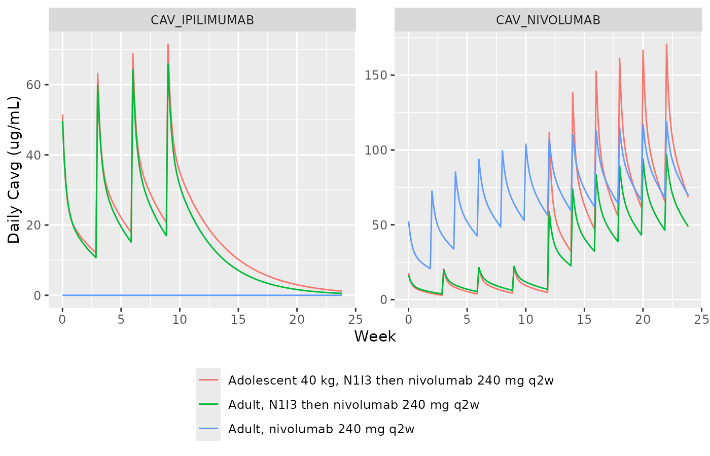
Typical daily Cavg of nivolumab and ipilimumab from the Hu 2024 population PK models, used as the time-varying exposure inputs of the Du 2024 hazard model.
The relative hazard is then evaluated day by day. The exposure-only part holds every baseline covariate at the reference patient; the total also applies each patient’s own age and weight.
hr_cov <- profiles |>
  mutate(.row = row_number())
exposure_only <- hr_eval(
  bind_rows(lapply(seq_len(nrow(hr_cov)), function(i) {
    scenario(CAV_NIVOLUMAB = hr_cov$CAV_NIVOLUMAB[i], CAV_IPILIMUMAB = hr_cov$CAV_IPILIMUMAB[i])
  }))
)
total <- hr_eval(
  bind_rows(lapply(seq_len(nrow(hr_cov)), function(i) {
    scenario(
      CAV_NIVOLUMAB = hr_cov$CAV_NIVOLUMAB[i], CAV_IPILIMUMAB = hr_cov$CAV_IPILIMUMAB[i],
      AGE = hr_cov$AGE[i], WT = hr_cov$WT[i]
    )
  }))
)
hr_time <- hr_cov |>
  mutate(`exposure only` = exposure_only, `exposure + age + weight` = total)

# Nivolumab monotherapy: the exposure term is close to flat (Figure 2b shows
# almost no spread of predicted probability across exposure percentiles).
mono <- filter(hr_time, regimen == "Adult, nivolumab 240 mg q2w")
stopifnot(all(mono$`exposure only` <= 1), all(mono$`exposure only` > 0.9))

# Age and weight alone put the 40 kg 15-year-old at exp(0.00414 * -45 +
# 0.006033 * -35) = 0.672 of the adult reference, an identity of the model.
adol <- filter(hr_time, regimen == "Adolescent 40 kg, N1I3 then nivolumab 240 mg q2w")
stopifnot(all(abs(adol$`exposure + age + weight` / adol$`exposure only` -
                    exp(0.00414 * -45 + 0.006033 * -35)) < 1e-6))
hr_time |>
  pivot_longer(c(`exposure only`, `exposure + age + weight`),
               names_to = "component", values_to = "hr") |>
  ggplot(aes(day / 7, hr, colour = regimen)) +
  geom_hline(yintercept = 1, colour = "grey60") +
  geom_line() +
  facet_wrap(~component) +
  labs(x = "Week", y = "Relative hazard", colour = NULL) +
  theme(legend.position = "bottom", legend.direction = "vertical")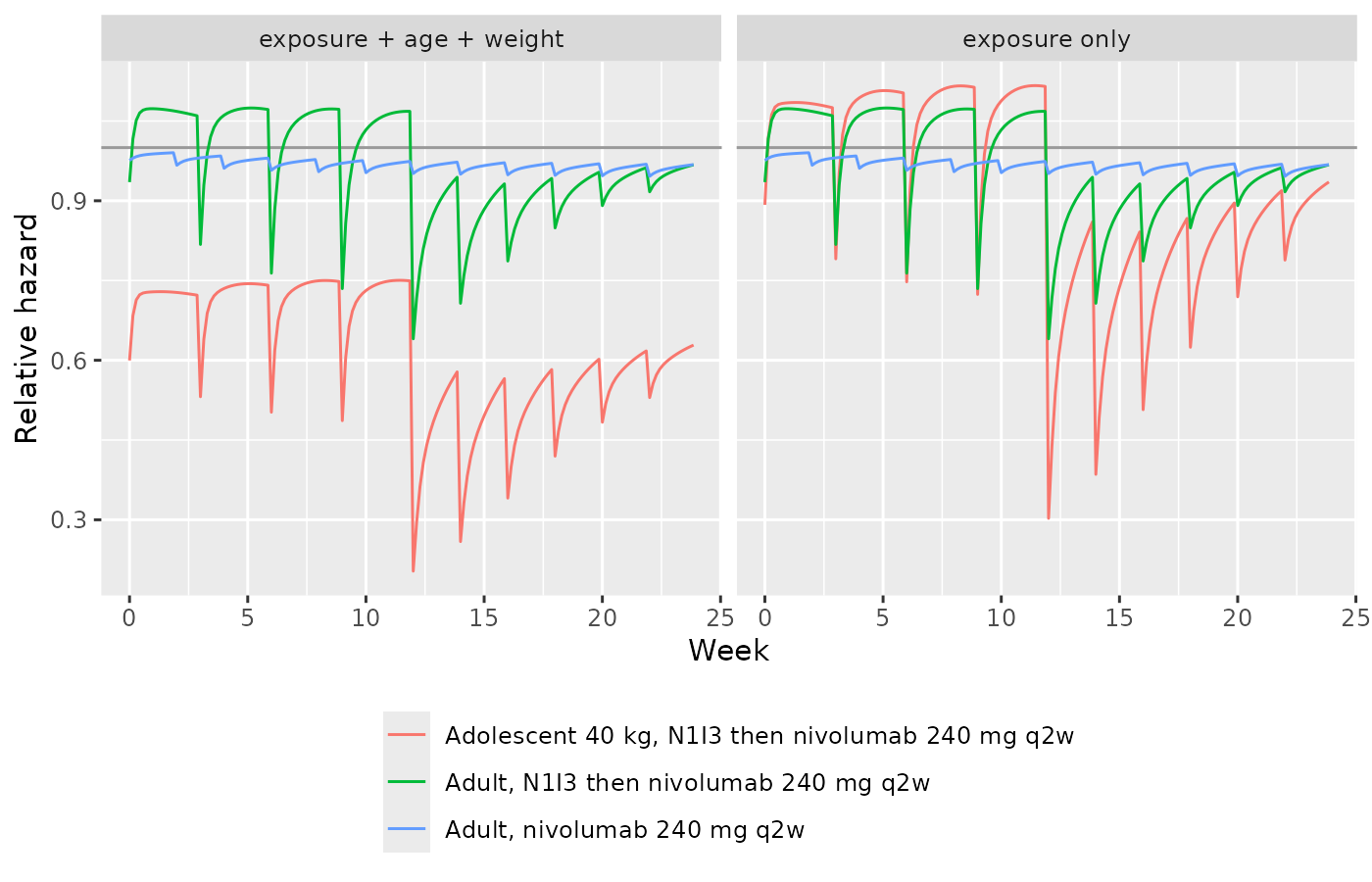
Relative hazard of a first gr2+ IMAE over the first 24 weeks, against the zero-exposure reference patient. Only ratios within one treatment stratum are meaningful: nivolumab monotherapy and the combination have different, unspecified baseline hazards.
For nivolumab monotherapy the exposure term barely moves the hazard (about 5% at the highest daily Cavg), which is the flat nivolumab exposure-response of Figure 2b. In combination the picture is set by the interaction. Early in induction, while nivolumab is still low, the ipilimumab term raises the hazard slightly; as nivolumab accumulates, the negative product term outweighs it, and the exposure-driven relative hazard falls below 1, most of all once flat 240 mg nivolumab maintenance starts while ipilimumab is still circulating. Within the combination stratum, the fitted surface therefore gives higher combined exposure a lower, not higher, relative hazard. This is a property of the linear-interaction form Du 2024 selected by BIC (Table S5). The paper reads it as a “synergistic effect” and as a relatively flat combination exposure-response. Do not use it to extrapolate beyond the exposures in the pooled studies.
For the adolescent, the lower age and weight alone cut the hazard by about a third, and the higher exposures from flat maintenance dosing do not raise it. That is the paper’s main conclusion: adolescents on the adult regimens are not predicted to carry a higher immune-mediated safety risk (Table 2, Figure 3).
Assumptions and deviations
- No baseline hazard. The model was fitted as a stratified Cox regression, so each treatment stratum has its own unspecified baseline hazard. The packaged model returns the relative hazard only, and the cumulative probabilities of Table 2, Figure 2 and Figure 3 cannot be simulated from it. Figure 2a plots baseline cumulative probabilities for the three strata, but its caption describes a reference patient (50 years) that differs from Figure 1’s (60 years), and a digitised step function would be a construction rather than a fitted quantity, so it was not encoded.
-
Centring. Age and weight are centred at the Figure
1 reference values (60 years, 75 kg), and the reference categories are
those of Figure 1. Centring a Cox model does not change any coefficient;
it only fixes what
hr = 1means. -
Line of therapy coding. The register’s
LINE_1Lis 1 for first line; the paper’s coefficient is for second or later line against first line, so the model applies it to1 - LINE_1L. The handling of the 23 patients with missing line of therapy is not described. -
PD-L1.
PDL1_TUM_POSmarks PD-L1 at or above the paper’s 5% threshold; the model switches it off whenPDL1_TUM_MISSING = 1, so the two indicators cannot both act. -
Exposure inputs.
CAV_NIVOLUMABandCAV_IPILIMUMABare daily averages (AUC over each calendar day divided by one day) in ug/mL, 0 when the antibody is not given. The illustration above takes them from the typical-value Hu 2024 models with 30-minute infusions and starts nivolumab maintenance three weeks after the fourth combination dose; Du 2024 used individual empirical-Bayes predictions. - Abstract body-weight figure. The abstract gives “0.84 for BW 52 kg versus 75 kg”. Table 1, Figure 1 and the Results text all give 0.87 for that contrast, which the model reproduces; 0.84 (0.844) is Figure 1’s age-P05 effect, so the abstract appears to have taken the neighbouring value.
- Figure 2 caption. The reference patient for Figures 2b and 2c lists “BLDHR = 10”, which is almost certainly 1 (the Figure 1 and Figure 2a reference). The difference matters little here: the LDH term would be exp(-0.0209 log 10) = 0.953.
- Table 2 combination rows. For the combination regimens with nivolumab 480 mg every 4 weeks maintenance, Table 2 prints cumulative probabilities that fall from 6 months to 1 year (for example 0.629 then 0.521 for adults), which a cumulative probability cannot do; those rows appear to be misaligned and are not used.
- Endpoint definition. For the ipilimumab-monotherapy studies the event is an immune-related adverse event, used in place of the IMAE definition (Table S2); the ipilimumab-monotherapy baseline hazard absorbs the difference.