Valproic acid syrup vs sustained-release tablets in children (Wang 2024)
Source:vignettes/articles/Wang_2024_valproic_acid.Rmd
Wang_2024_valproic_acid.RmdModel and source
Wang et al. (2024) developed a one-compartment population pharmacokinetic model with first-order absorption for total plasma valproic acid (VPA) in children with epilepsy, from 1411 routine therapeutic-drug-monitoring (TDM) trough concentrations in 617 patients at a single centre in Nanjing, China. The question the paper is built around is a practical one: VPA syrup and sustained-release (SR) tablets are not interchangeable milligram for milligram, so how should the dose be changed when a child is switched from one to the other?
The final model is:
with Sex = 0 for male and Sex = 1 for
female, and with the absorption rate constant FIXED by formulation at
ka = 2.64 1/h for syrup and ka = 0.46 1/h for
SR tablets.
Two features of this model are worth flagging before any simulation, because both are consequences of a trough-only TDM dataset rather than modelling choices:
-
Both
kavalues are fixed from the literature, not estimated. The dataset contains no absorption-phase samples, so absorption is unidentifiable from it. The 2.64 / 0.46 pair is a valproate-literature convention that this paper takes from Mei 2018 and that the siblingZhang_2023_*andZhang_2024_valproic_acidmodels take from Ding 2015. -
There is no interindividual variability on
V/F. It “was not informative enough to be calculated because only the Ctrough samples of VPA were available, and then were excluded from the model.”
mod <- modellib("Wang_2024_valproic_acid")
mod
#> function() {
#>   description <- "One-compartment population PK model with first-order absorption for total plasma valproic acid in Chinese children with epilepsy (Wang 2024 final model), built to tailor the dose when switching between oral syrup and sustained-release tablets. Apparent clearance carries a power body-weight effect and a proportional female-sex effect; apparent volume carries a power body-weight effect. Formulation-specific absorption rate constants are FIXED from the literature (oral syrup 2.64 1/h reference, sustained-release tablet 0.46 1/h), because the therapeutic-drug-monitoring dataset is steady-state troughs only and contains no absorption-phase data."
#>   reference <- paste(
#>     "Wang WJ, Li Y, Hu YH, Wang J, Zhang YY, Fan L, Dai HR, Guo HL, Ding XS,",
#>     "Chen F. Population pharmacokinetics of valproic acid in children with",
#>     "epilepsy: Implications for dose tailoring when switching from oral syrup",
#>     "to sustained-release tablets. CPT Pharmacometrics Syst Pharmacol.",
#>     "2024;13(9):1554-1569. doi:10.1002/psp4.13191. PMCID PMC11533106.",
#>     "Final-model parameter estimates from Table 3; covariate equations from",
#>     "Equations 34 and 35.",
#>     sep = " "
#>   )
#>   vignette <- "Wang_2024_valproic_acid"
#>   units <- list(time = "h", dosing = "mg", concentration = "mg/L")
#>
#>   # Issue #482: what each ODE state holds, in what amount units, in what
#>   # biological matrix.
#>   compartmentData <- list(
#>     depot = list(analyte = "valproic acid", units = "mg", specimen = "administration site", verified = TRUE),
#>     central = list(analyte = "valproic acid", units = "mg", specimen = "plasma", verified = TRUE)
#>   )
#>
#>   covariateData <- list(
#>     WT = list(
#>       description = "Body weight",
#>       units = "kg",
#>       type = "continuous",
#>       reference_category = "22 kg (the model-development cohort median; Wang 2024 Table 2)",
#>       notes = "Power effect on both CL/F (exponent 0.717) and V/F (exponent 0.524), each normalised to the 22.0 kg cohort median. Cohort range 6.0-95.0 kg (Wang 2024 Table 2). The authors compared five body-weight / age scaling forms (fixed allometric, simple exponent, sigmoid maturation, body-weight-dependent exponent, age-dependent exponent; Methods Equations 6-13) and selected the SIMPLE EXPONENT model (Model II) with both exponents estimated: the two dependent-exponent models fitted better on OFV/AIC but their kmax and Hill terms had RSE > 60%, and TM50/kmax/Hill could not be estimated at all in the sigmoid maturation model. Note the estimated CL/F exponent 0.717 is close to, but was NOT fixed at, the allometric 0.75. Age is not in the final model because it correlates with body weight at r = 0.948 in this cohort (Wang 2024 Discussion).",
#>       source_name = "BW"
#>     ),
#>     SEXF = list(
#>       description = "Female sex indicator",
#>       units = "(binary)",
#>       type = "binary",
#>       reference_category = "0 (male)",
#>       notes = "PROPORTIONAL (not exponential) effect on CL/F: the paper's Equation 34 is CL/F = 0.196 * (BW/22)^0.717 * (1 - 0.0436 * Sex) with 'Sex = 0 for male, Sex = 1 for female' stated immediately below the equation, so the paper's Sex indicator is already the canonical SEXF orientation and needs no recoding. Females therefore have 4.36% LOWER apparent clearance and hence 1/(1 - 0.0436) = 4.6% HIGHER exposure at an equivalent dose, which matches the Discussion's 'Compared with males, females exhibited 5-10% higher exposure of VPA at equivalent dose (Figure 2)'. Note the DIRECTION is opposite to the sibling Zhang_2024_valproic_acid.R, where women had 12.9% higher clearance; Zhang attributes its direction to the larger median body weight of the women in that adult-inclusive cohort. 194 of 498 model-development patients (39.0%) were female (Wang 2024 Table 2). Sex was retained on the strength of an OFV drop of 11.727 (p < 0.001) over the covariate-free Model II.",
#>       source_name = "Sex"
#>     ),
#>     FORM_VPA_SR = list(
#>       description = "Sustained-release valproic acid tablet formulation indicator",
#>       units = "(binary)",
#>       type = "binary",
#>       reference_category = "0 (oral syrup, the reference formulation in this cohort)",
#>       notes = "Selects the FIXED sustained-release-tablet absorption rate constant Ka = 0.46 1/h; the oral-syrup reference is Ka = 2.64 1/h. Wang 2024 Methods, Base model: 'The fixed values for ka were 2.64 and 0.46 h-1 for syrup and SR tablets, respectively, due to a lack of absorption phase data', citing Mei 2018 (reference 19) - the same literature Ka pair that Zhang_2023_* and Zhang_2024_valproic_acid.R trace to Ding 2015. This cohort has only the two levels syrup and sustained-release tablet, so FORM_TABLET (the conventional immediate-release level used by Zhang_2023_valproic_acid_base.R) is not part of this model. Across the full 617-patient cohort 471 patients received syrup and 154 received SR tablets; 8 patients started on syrup and later switched, which is why the Table 2 per-arm percentages sum to slightly more than 100%.",
#>       source_name = "Dosage forms"
#>     )
#>   )
#>
#>   covariatesDataExcluded <- list(
#>     AGE = list(
#>       description = "Age",
#>       units = "years",
#>       type = "continuous",
#>       notes = "Median 5.8 years, range 0.2-17.2 (Wang 2024 Table 2). Screened as a maturation covariate on CL/F in Models III (sigmoid maturation) and V (age-dependent exponent) but NOT retained: TM50, kmax and Hill 'were failed to be estimated in our study' (Discussion), and the strong body-weight/age correlation (r = 0.948) 'necessitates the exclusion of one of these variables, leading to the simplification of the model into a basic exponent model'."
#>     ),
#>     DOSE_VPA_MGKGD = list(
#>       description = "Total daily valproic acid dose per kg body weight",
#>       units = "mg/kg/d",
#>       type = "continuous",
#>       notes = "Median 21.7 mg/kg/day, range 7.7-40.0 (Wang 2024 Table 2). Screened as a surrogate for concentration-dependent protein-binding saturation in Models VI (TDD simple exponent) and VII (dose-dependent Emax, with Emax and Hill fixed at 2.8 and 1.68 from Ding 2015). Model VII did lower the OFV to 7037.671, below the retained Model II, but was rejected because its typical CL/F of 0.052 L/h was 'unreasonable'. The Discussion further cautions that incorporating TDD in a therapeutic-drug-monitoring dataset is confounded by the TDM feedback effect. No nonlinear protein-binding term appears in the final model.",
#>       source_name = "TDD"
#>     ),
#>     ALB = list(
#>       description = "Serum albumin",
#>       units = "g/L",
#>       type = "continuous",
#>       notes = "Screened by forward inclusion as a continuous covariate on CL/F in linear, power and exponential forms (Methods Equations 23-25) and not retained. Albumin also enters Models VIII-X, the three explicit protein-binding models (one-binding-site with K = 15.5 1/mM and N = 1.98; Langmuir with Kd = 7.8 and Bm = 130 mg/L; linear non-saturable with Kd = 2.12, Bm = 67.3 mg/L and NS = 2.25), none of which improved on the linear Model II. Per-patient values are in Table S1, which is not reproduced in the main text."
#>     ),
#>     ALT = list(
#>       description = "Alanine aminotransferase",
#>       units = "U/L",
#>       type = "continuous",
#>       notes = "Screened by forward inclusion as a hepatic-function covariate on CL/F and not retained (Wang 2024 Methods, Covariate model). Per-patient values are in Table S1, which is not reproduced in the main text."
#>     ),
#>     AST = list(
#>       description = "Aspartate aminotransferase",
#>       units = "U/L",
#>       type = "continuous",
#>       notes = "Screened by forward inclusion as a hepatic-function covariate on CL/F and not retained (Wang 2024 Methods, Covariate model). Per-patient values are in Table S1, which is not reproduced in the main text."
#>     ),
#>     CREAT = list(
#>       description = "Serum creatinine",
#>       units = "umol/L",
#>       type = "continuous",
#>       notes = "A negative correlation with CL/F was seen during covariate evaluation but creatinine was NOT retained. The Discussion rejects it on physiological grounds: the patients' creatinine was almost entirely within the age-appropriate reference range, valproic acid is rarely excreted unchanged in urine, and creatinine 'is not a reliable surrogate for estimating the renal function in children' because it tracks muscle mass (Figure S4)."
#>     ),
#>     CYSC = list(
#>       description = "Serum cystatin C",
#>       units = "mg/L",
#>       type = "continuous",
#>       notes = "Used in place of creatinine to derive the estimated glomerular filtration rate, because the study recorded no height and so could not apply a height-based paediatric equation. Not itself retained on CL/F.",
#>       source_name = "CysC"
#>     ),
#>     CRCL = list(
#>       description = "Estimated glomerular filtration rate",
#>       units = "mL/min/1.73 m^2",
#>       type = "continuous",
#>       notes = "Derived three ways (Methods Equations 20-22: the KDIGO 2012 cystatin-C equation, Shull's equation, and a further cystatin-C-based equation) and screened on CL/F. 'Renal function did not impact VPA's CL/F' (Results, Covariate model); the Discussion adds that the KDIGO 2012 cystatin-C eGFR 'did not fulfill the inclusion/exclusion criteria'. The canonical column CRCL is the register's home for a renal-function covariate reported as an eGFR in mL/min/1.73 m^2; this model does not use it.",
#>       source_name = "eGFR"
#>     ),
#>     CONMED_OXC = list(
#>       description = "Concomitant oxcarbazepine indicator",
#>       units = "(binary)",
#>       type = "binary",
#>       notes = "39 of 498 model-development patients (7.8%). Reached forward-inclusion significance on CL/F with an OFV drop of 7.981 (p < 0.05) but was removed in backward elimination (dOFV < 10.83). The Discussion attributes the non-retention to the small number of co-treated subjects.",
#>       source_name = "OXC"
#>     ),
#>     CONMED_LAMOTRIGINE = list(
#>       description = "Concomitant lamotrigine indicator",
#>       units = "(binary)",
#>       type = "binary",
#>       notes = "55 of 498 model-development patients (11.0%). Forward-inclusion OFV drop of 8.329 (p < 0.05) on CL/F; removed in backward elimination (dOFV < 10.83).",
#>       source_name = "LTG"
#>     ),
#>     CONMED_CZP = list(
#>       description = "Concomitant clonazepam indicator",
#>       units = "(binary)",
#>       type = "binary",
#>       notes = "39 of 498 model-development patients (7.8%). Forward-inclusion OFV drop of 7.049 (p < 0.05) on CL/F; removed in backward elimination (dOFV < 10.83).",
#>       source_name = "CZP"
#>     ),
#>     CONMED_PB = list(
#>       description = "Concomitant phenobarbital indicator",
#>       units = "(binary)",
#>       type = "binary",
#>       notes = "Only 1 of 498 model-development patients (0.2%), so phenobarbital fell below the paper's own '>5% of patients' screening threshold. The Discussion nonetheless reports a forward-inclusion OFV drop of 8.602 for concurrent phenobarbital therapy; it was removed in backward elimination.",
#>       source_name = "PB"
#>     ),
#>     CONMED_TPM = list(
#>       description = "Concomitant topiramate indicator",
#>       units = "(binary)",
#>       type = "binary",
#>       notes = "51 of 498 model-development patients (10.2%), so topiramate passed the '>5% of patients' threshold and was screened as a covariate on CL/F, but the paper reports no OFV drop for it and it is not retained. 'In this study, little impact of concurrent ASMs on VPA's CL/F was observed.'",
#>       source_name = "TPM"
#>     )
#>   )
#>
#>   population <- list(
#>     species = "human",
#>     n_subjects = 498,
#>     n_studies = 1,
#>     n_observations = 1138,
#>     age_range = "0.2-17.2 years",
#>     age_median = "5.8 years",
#>     weight_range = "6.0-95.0 kg",
#>     weight_median = "22.0 kg",
#>     sex_female_pct = 39.0,
#>     race_ethnicity = "Chinese (single-centre Nanjing cohort; sub-ethnicity not reported)",
#>     disease_state = "Epilepsy, treated with valproic acid for at least 1 week before sampling",
#>     dose_range = "7.7-40.0 mg/kg/day (median 21.7), given one to three times daily as oral syrup or sustained-release tablet",
#>     regions = "China (Children's Hospital of Nanjing Medical University; January 2022 - March 2023)",
#>     co_medication = "Concomitant antiseizure medications in the model-development set: levetiracetam 102 (20.5%), lamotrigine 55 (11.0%), topiramate 51 (10.2%), clonazepam 39 (7.8%), oxcarbazepine 39 (7.8%), perampanel 35 (7.0%), lacosamide 23 (4.6%), vigabatrin 5 (1.0%), zonisamide 5 (1.0%), phenobarbital 1 (0.2%). Only co-medications used by more than 5% of patients were screened as covariates, and none was retained in the final model. Patients taking any non-antiseizure co-medication were excluded at enrolment.",
#>     notes = "1411 steady-state trough concentrations from 617 children were split 8:2 into a model-development set (498 patients, 1138 samples) and an external-evaluation set (119 patients, 273 samples); the numbers recorded in this metadata block are the MODEL-DEVELOPMENT set, which is what Table 3 was fitted to. External-evaluation set: 119 patients (78 male / 41 female), age median 6.2 years (0.5-13.8), body weight median 23.0 kg (6.0-75.0). Observed valproic acid concentrations 12.6-143.1 mg/L (median 68.6), all routine therapeutic-drug-monitoring TROUGHS - there is no absorption-phase sampling, which is why both Ka values are fixed from the literature and why interindividual variability on V/F 'was not informative enough to be calculated' and was dropped. Assay: enzyme multiplied immunoassay technique (EMIT; Viva-E, Siemens), calibration range 1.00-150 mg/L, within- and between-run coefficients of variation below 15%. Median 2 samples per patient (range 1-9). Model fitted in NONMEM 7.3.0 with PsN 5.2.6 using FOCE-I and the ADVAN2 TRANS2 subroutines. Baseline demographics: Wang 2024 Table 2."
#>   )
#>
#>   ini({
#>     # ----------------------------------------------------------------
#>     # Absorption - FIXED to the literature Ka pair the authors adopted.
#>     # Wang 2024 Methods, Base model: "The fixed values for ka were 2.64
#>     # and 0.46 h-1 for syrup and SR tablets, respectively, due to a lack
#>     # of absorption phase data." Oral syrup is the reference
#>     # formulation, so lka is the syrup value and the SR indicator
#>     # carries the log-ratio shift (the same pattern as the sibling
#>     # Zhang_2024_valproic_acid.R, which fixes the identical pair).
#>     # ----------------------------------------------------------------
#>     lka <- fixed(log(2.64)); label("Absorption rate constant, oral syrup reference (1/h)")                                # Wang 2024 Methods Base model and Table 3 (Ka1 = 2.64, Fixed)
#>     e_form_vpa_sr_ka <- fixed(log(0.46 / 2.64)); label("Log-ratio shift on Ka for sustained-release tablet vs oral syrup") # Wang 2024 Methods Base model and Table 3 (Ka2 = 0.46, Fixed)
#>
#>     # ----------------------------------------------------------------
#>     # Structural parameters, final model. Both are apparent (oral)
#>     # parameters describing TOTAL plasma valproic acid: "as
#>     # bioavailability (F) could not be determined, the CL and the Vd
#>     # were considered as the apparent CL (CL/F) and Vd (Vd/F)".
#>     #
#>     # Cross-check on the reference weight: at BW = 22 kg these give
#>     # CL/F = 0.196 / 22 = 0.0089 L/h/kg and V/F = 2.09 / 22 = 0.095
#>     # L/kg, which is exactly the paper's own summary immediately below
#>     # Equation 35 ("the typical value for the CL/F of VPA in children
#>     # at steady state obtained in our study was 0.009 L/h/kg and the
#>     # V/F was 0.1 L/kg"). This confirms 22 kg is the normalising
#>     # weight, which Equations 34-35 write only as the literal "22".
#>     # ----------------------------------------------------------------
#>     lcl <- log(0.196); label("Apparent clearance CL/F for a 22 kg male (L/h)")            # Wang 2024 Table 3 final model (CL/F = 0.196 L/h, RSE 3%, bootstrap 95% CI [0.183, 0.208]) and Equation 34
#>     lvc <- log(2.09);  label("Apparent volume of distribution V/F at 22 kg (L)")          # Wang 2024 Table 3 final model (V/F = 2.09 L, RSE 9%, bootstrap 95% CI [1.69, 2.49]) and Equation 35
#>
#>     # ----------------------------------------------------------------
#>     # Covariate effects. Wang 2024 Equations 34 and 35:
#>     #   CL/F = 0.196 * (BW/22)^0.717 * (1 - 0.0436 * Sex)
#>     #   V/F  = 2.09  * (BW/22)^0.524
#>     # with "Sex = 0 for male, Sex = 1 for female".
#>     #
#>     # NOTE the sex term is the paper's PROPORTIONAL categorical form
#>     # (Methods Equation 27, Pi = TV(P) * (1 + theta * COV)), NOT the
#>     # exponential form (Equation 28). It is therefore applied as a
#>     # multiplicative (1 + e_sexf_cl * SEXF) factor in model() rather
#>     # than folded into the log-scale sum, so the encoded value is
#>     # exactly the tabulated -0.0436 with no back-transformation.
#>     # ----------------------------------------------------------------
#>     e_wt_cl   <-  0.717;   label("Power exponent on (WT/22) for CL/F (unitless)")         # Wang 2024 Table 3 "BW on CL/F" 0.717 (RSE 4%, bootstrap 95% CI [0.659, 0.775]); Equation 34
#>     e_wt_vc   <-  0.524;   label("Power exponent on (WT/22) for V/F (unitless)")          # Wang 2024 Table 3 "BW on V/F" 0.524 (RSE 15%, bootstrap 95% CI [0.361, 0.686]); Equation 35
#>     e_sexf_cl <- -0.0436;  label("Proportional shift on CL/F for female sex (unitless)")  # Wang 2024 Table 3 "Sex on CL/F" -0.0436 (RSE 29%, bootstrap 95% CI [-0.0685, -0.0187]); Equation 34
#>
#>     # ----------------------------------------------------------------
#>     # IIV. Wang 2024 Table 3 reports a single "IIV on CL/F (%)" of
#>     # 11.9 (RSE 6%, bootstrap 95% CI [10.4, 13.2]) under the
#>     # exponential IIV model of Equation 1. The IIV on V/F "was not
#>     # informative enough to be calculated because only the Ctrough
#>     # samples of VPA were available, and then were excluded from the
#>     # model" (Results, Base model).
#>     #
#>     # The tabulated 11.9 is a CV%, so the internal variance is
#>     #   omega^2 = log(CV^2 + 1) = log(0.119^2 + 1) = 0.014062
#>     #
#>     # This is a load-bearing reading, because a variance-scale reading
#>     # (omega^2 = 0.119, i.e. CV = 35.5%) is also superficially
#>     # available. It is settled by the authors' own Figure 2, whose
#>     # boxes are "the median and IQR of Ctrough for each dosing
#>     # regimen" over 1000 simulated patients: the drawn boxes have
#>     # Q3/Q1 of roughly 1.2 (e.g. the 20 kg male / 40 mg/kg/day syrup
#>     # box spans about 92-112 mg/L about a median near 102), which for
#>     # a log-normal implies a log-scale SD near 0.15 - consistent with
#>     # a 11.9% CV plus this model's residual error, and flatly
#>     # inconsistent with a 35.5% CV, which would put the same panel's
#>     # Tukey whiskers below 10 and above 190 mg/L instead of the drawn
#>     # 75-140 mg/L.
#>     #
#>     # The zero-variance V/F term is OMITTED rather than written as
#>     # `etalvc ~ fixed(0)`: a zero diagonal makes OMEGA singular and
#>     # breaks the Cholesky sampler used by rxSolve (same treatment as
#>     # the sibling Zhang_2024_valproic_acid.R).
#>     # ----------------------------------------------------------------
#>     etalcl ~ 0.014062  # Wang 2024 Table 3 final model (IIV on CL/F = 11.9%, exponential per Equation 1)
#>
#>     # ----------------------------------------------------------------
#>     # Residual variability - combined proportional and additive. Wang
#>     # 2024 Results, Base model: "The combined additive and proportional
#>     # model (Equation 5) showed the best fit for characterizing the
#>     # RV". Table 3 tabulates RVprop = 0.0151 (RSE 15%) and RVadd = 22.6
#>     # (RSE 35%), which are NONMEM $SIGMA VARIANCES, so the standard
#>     # deviations this file encodes are
#>     #   propSd = sqrt(0.0151) = 0.12288      (12.3%)
#>     #   addSd  = sqrt(22.6)   = 4.7539 mg/L
#>     #
#>     # The variance reading is confirmed by the assay: combining the two
#>     # at the cohort median trough of 68.6 mg/L gives
#>     #   sqrt((0.12288 * 68.6)^2 + 4.7539^2) / 68.6 = 14.1%
#>     # against an EMIT assay whose within- and between-run coefficients
#>     # of variation are "below 15%" (Methods, Bioassay of VPA). Reading
#>     # the tabulated numbers as standard deviations instead would put
#>     # the additive term alone at 22.6 mg/L, i.e. 33% of the median
#>     # trough, which no assay-limited TDM dataset supports.
#>     #
#>     # Equation 5 is TYPESET as Y = IPRED * (1 + eps1 + eps2), which
#>     # would make BOTH error terms proportional. That contradicts Table
#>     # 3's own row labels ("RVprop" and "RVadd") and is arithmetically
#>     # impossible for the tabulated magnitude - a proportional variance
#>     # of 22.6 is a 475% CV. It is a typesetting slip for the standard
#>     # NONMEM combined form Y = IPRED * (1 + eps1) + eps2, which is what
#>     # is encoded here.
#>     # ----------------------------------------------------------------
#>     propSd <- 0.12288; label("Proportional residual SD (fraction)")   # Wang 2024 Table 3 final model (RVprop = 0.0151 variance, RSE 15%, bootstrap 95% CI [0.0105, 0.0198])
#>     addSd  <- 4.7539;  label("Additive residual SD (mg/L)")           # Wang 2024 Table 3 final model (RVadd = 22.6 variance, RSE 35%, bootstrap 95% CI [6.58, 38.5])
#>   })
#>
#>   model({
#>     # 1. Formulation-specific absorption rate constant. Oral syrup is
#>     #    the reference (FORM_VPA_SR = 0); both values are FIXED.
#>     ka <- exp(lka + e_form_vpa_sr_ka * FORM_VPA_SR)
#>
#>     # 2. Apparent clearance, Equation 34. The body-weight power term is
#>     #    written on the log scale (exponent * log(ratio)), which is
#>     #    algebraically identical to the paper's (BW/22)^0.717 form; the
#>     #    sex term stays OUTSIDE the exponential because the paper uses
#>     #    the proportional categorical model (1 - 0.0436 * Sex), not the
#>     #    exponential one.
#>     cl <- exp(lcl + e_wt_cl * log(WT / 22) + etalcl) * (1 + e_sexf_cl * SEXF)
#>
#>     # 3. Apparent volume of distribution, Equation 35. No
#>     #    interindividual variability (not estimable from trough-only
#>     #    data; see ini()).
#>     vc <- exp(lvc + e_wt_vc * log(WT / 22))
#>
#>     # 4. Micro-constant
#>     kel <- cl / vc
#>
#>     # 5. One-compartment ODE system with first-order oral absorption
#>     #    (NONMEM ADVAN2 TRANS2)
#>     d/dt(depot)   <- -ka * depot
#>     d/dt(central) <-  ka * depot - kel * central
#>
#>     # 6. Observation (total plasma valproic acid) and residual error
#>     Cc <- central / vc
#>     Cc ~ prop(propSd) + add(addSd)
#>   })
#> }
#> <environment: 0x5581de869288>

# Parsed once here so the metadata lists below can be read off the model file
# itself. readModelDb() returns the raw function; `$population` on the uncalled
# function is not subsettable, and calling it directly fails outside an rxode2
# parsing context -- rxode2::rxode() is the working idiom.
mod_meta <- rxode2::rxode(readModelDb("Wang_2024_valproic_acid"))
#> ℹ parameter labels from comments will be replaced by 'label()'
Population
| Field | Value |
|---|---|
| species | human |
| n_subjects | 498 |
| n_studies | 1 |
| n_observations | 1138 |
| age_range | 0.2-17.2 years |
| age_median | 5.8 years |
| weight_range | 6.0-95.0 kg |
| weight_median | 22.0 kg |
| sex_female_pct | 39 |
| race_ethnicity | Chinese (single-centre Nanjing cohort; sub-ethnicity not reported) |
| disease_state | Epilepsy, treated with valproic acid for at least 1 week before sampling |
| dose_range | 7.7-40.0 mg/kg/day (median 21.7), given one to three times daily as oral syrup or sustained-release tablet |
| regions | China (Children’s Hospital of Nanjing Medical University; January 2022 - March 2023) |
| co_medication | Concomitant antiseizure medications in the model-development set: levetiracetam 102 (20.5%), lamotrigine 55 (11.0%), topiramate 51 (10.2%), clonazepam 39 (7.8%), oxcarbazepine 39 (7.8%), perampanel 35 (7.0%), lacosamide 23 (4.6%), vigabatrin 5 (1.0%), zonisamide 5 (1.0%), phenobarbital 1 (0.2%). Only co-medications used by more than 5% of patients were screened as covariates, and none was retained in the final model. Patients taking any non-antiseizure co-medication were excluded at enrolment. |
| notes | 1411 steady-state trough concentrations from 617 children were split 8:2 into a model-development set (498 patients, 1138 samples) and an external-evaluation set (119 patients, 273 samples); the numbers recorded in this metadata block are the MODEL-DEVELOPMENT set, which is what Table 3 was fitted to. External-evaluation set: 119 patients (78 male / 41 female), age median 6.2 years (0.5-13.8), body weight median 23.0 kg (6.0-75.0). Observed valproic acid concentrations 12.6-143.1 mg/L (median 68.6), all routine therapeutic-drug-monitoring TROUGHS - there is no absorption-phase sampling, which is why both Ka values are fixed from the literature and why interindividual variability on V/F ‘was not informative enough to be calculated’ and was dropped. Assay: enzyme multiplied immunoassay technique (EMIT; Viva-E, Siemens), calibration range 1.00-150 mg/L, within- and between-run coefficients of variation below 15%. Median 2 samples per patient (range 1-9). Model fitted in NONMEM 7.3.0 with PsN 5.2.6 using FOCE-I and the ADVAN2 TRANS2 subroutines. Baseline demographics: Wang 2024 Table 2. |
The metadata above describes the model-development set (498 patients, 1138 samples), which is what Table 3 was fitted to; a further 119 patients with 273 samples were held out for external evaluation. The cohort is young and light – median age 5.8 years, median body weight 22.0 kg – and every sample is a steady-state trough drawn under routine TDM.
Source trace
Every value in the model file, with the location it came from.
| Quantity | Value | Source |
|---|---|---|
| Structural model | 1-compartment, first-order absorption (NONMEM ADVAN2 TRANS2) | Methods, Base model; Results, Base model |
| ODE: depot | d(depot)/dt = -ka * depot | Methods, Base model (ADVAN2 TRANS2) |
| ODE: central | d(central)/dt = ka * depot - kel * central | Methods, Base model (ADVAN2 TRANS2) |
| Observation | Cc = central / vc | Methods, Base model |
| Ka (oral syrup) | 2.64 1/h, FIXED | Methods, Base model; Table 3 (Ka1, ‘Fixed’); from Mei 2018 (ref. 19) |
| Ka (SR tablet) | 0.46 1/h, FIXED | Methods, Base model; Table 3 (Ka2, ‘Fixed’); from Mei 2018 (ref. 19) |
| CL/F typical | 0.196 L/h at 22 kg, male | Equation 34; Table 3 (0.196, RSE 3%, CI [0.183, 0.208]) |
| V/F typical | 2.09 L at 22 kg | Equation 35; Table 3 (2.09, RSE 9%, CI [1.69, 2.49]) |
| BW normalising value | 22 kg (cohort median) | Equations 34-35 (literal ‘22’); Table 2 (BW median 22.0 kg) |
| BW exponent on CL/F | 0.717 | Equation 34; Table 3 (‘BW on CL/F’, RSE 4%, CI [0.659, 0.775]) |
| BW exponent on V/F | 0.524 | Equation 35; Table 3 (‘BW on V/F’, RSE 15%, CI [0.361, 0.686]) |
| Female sex on CL/F | -0.0436, PROPORTIONAL (1 - 0.0436 * Sex) | Equation 34; Table 3 (‘Sex on CL/F’, RSE 29%, CI [-0.0685, -0.0187]) |
| Sex coding | Sex = 0 male, Sex = 1 female | Stated immediately below Equation 35 |
| IIV on CL/F | 11.9% CV -> omega^2 = log(CV^2+1) = 0.014062 | Table 3 (‘IIV on CL/F (%)’, RSE 6%, CI [10.4, 13.2]); Equation 1 |
| IIV on V/F | not estimated; term omitted | Results, Base model (‘not informative enough to be calculated’) |
| Residual error | combined proportional + additive | Results, Base model (Equation 5 best fit) |
| RV proportional | variance 0.0151 -> propSd = 0.12288 | Table 3 (‘RVprop’, RSE 15%, CI [0.0105, 0.0198]) |
| RV additive | variance 22.6 -> addSd = 4.7539 mg/L | Table 3 (‘RVadd’, RSE 35%, CI [6.58, 38.5]) |
Three transcription decisions in this model are load-bearing and are recorded here in full, because each had a superficially plausible alternative.
1. The sex effect is proportional, not exponential.
The paper offers both forms in its Methods (Equation 27 proportional,
Equation 28 exponential) and Equation 34 uses the proportional one:
(1 - 0.0436 * Sex). The model file therefore applies the
sex term as a multiplicative factor outside the
exponential, so the encoded number is exactly the tabulated
-0.0436 with no back-transformation. Encoding it as
exp(-0.0436) would be a 0.1% error here, but it would be
the wrong functional form.
2. IIV on CL/F (%) = 11.9 is a CV%, not a
variance. This matters: read as a variance it would imply a
35.5% CV, a threefold difference. It is settled by the authors’ own
Figure 2, whose boxes are “the median and IQR of Ctrough for
each dosing regimen” over their simulated patients. The drawn boxes have
a Q3/Q1 ratio near 1.2 – for instance the 20 kg male / 40 mg/kg/day
syrup box spans roughly 92-112 mg/L about a median near 102 – which for
a log-normal implies a log-scale SD near 0.15. That is consistent with
an 11.9% CV plus this model’s residual error, and flatly inconsistent
with a 35.5% CV, which would place the same panel’s Tukey whiskers below
10 and above 190 mg/L instead of the drawn 75-140 mg/L.
3. RVprop and RVadd are NONMEM
variances. Table 3 gives 0.0151 and 22.6; the model file
encodes their square roots, 0.12288 and 4.7539 mg/L. The check is the
assay: combining the two at the cohort median trough of 68.6 mg/L gives
sqrt((0.12288 * 68.6)^2 + 4.7539^2) / 68.6 = 14.1%, against
an EMIT assay whose within- and between-run coefficients of variation
are “below 15%”. Reading them as standard deviations instead would put
the additive term alone at 22.6 mg/L, a third of the median trough,
which no assay-limited TDM dataset supports.
Separately, Equation 5 is typeset as
Y = IPRED * (1 + eps1 + eps2), which would make both error
terms proportional. That contradicts Table 3’s own row labels
(RVprop, RVadd) and is arithmetically
impossible at the tabulated magnitude – a proportional variance of 22.6
is a 475% CV. It is read here as a typesetting slip for the standard
NONMEM combined form Y = IPRED * (1 + eps1) + eps2.
Verification
Throughout this section tau = 12 h, matching the paper’s
own simulations (“doses ranging from 10 to 40 mg/kg/day per 12 h”).
tau <- 12

# Add the model's covariates to an rxode2 event table. Covariates MUST be
# attached after as.data.frame() -- assigning columns onto an rxEt object is
# silently dropped by rxode2.
add_cov <- function(ev, WT, SEXF, FORM_VPA_SR) {
  d <- as.data.frame(ev)
  d$WT <- WT
  d$SEXF <- SEXF
  d$FORM_VPA_SR <- FORM_VPA_SR
  d
}
The model reproduces the paper’s own per-kg summary
Immediately below Equation 35 the authors summarise their typical
patient: “the typical value for the CL/F of VPA in children at steady
state obtained in our study was 0.009 L/h/kg and the V/F was 0.1 L/kg”.
Dividing the tabulated CL/F and V/F by the
normalising weight must recover exactly that. This is also what confirms
the literal “22” in Equations 34-35 is the 22.0 kg cohort median from
Table 2, rather than some other reference weight.
per_kg <- tibble::tibble(
  Parameter = c("CL/F", "V/F"),
  `Typical value at 22 kg` = c(0.196, 2.09),
  `Per kg` = c(0.196 / 22, 2.09 / 22),
  `Paper's stated per-kg value` = c(0.009, 0.1)
)

knitr::kable(per_kg, digits = 6,
caption = "Per-kg typical values against the paper's own prose.")| Parameter | Typical value at 22 kg | Per kg | Paper’s stated per-kg value |
|---|---|---|---|
| CL/F | 0.196 | 0.008909 | 0.009 |
| V/F | 2.090 | 0.095000 | 0.100 |
The solved model reproduces a closed-form steady-state trough
For a one-compartment first-order-absorption model the steady-state
concentration at the end of a dosing interval has a closed form.
Comparing it against rxSolve on the packaged model
exercises every transcribed value at once – both ka values,
CL/F, V/F, both body-weight exponents, the
reference weight and the sex term. Because the two sides use the
same parameters and differ only by numerical integration, a
tight bound is the correct assertion here.
ctrough_closed_form <- function(BW, SEXF, mgkgd, sr) {
  cl <- 0.196 * (BW / 22)^0.717 * (1 - 0.0436 * SEXF)
  vc <- 2.09 * (BW / 22)^0.524
  ka <- if (sr) 0.46 else 2.64
  kel <- cl / vc
  D <- BW * mgkgd / 2                      # q12h => half the daily dose
  (D * ka / (vc * (ka - kel))) *
    (exp(-kel * tau) / (1 - exp(-kel * tau)) -
       exp(-ka * tau) / (1 - exp(-ka * tau)))
}

ctrough_solved <- function(BW, SEXF, mgkgd, sr) {
  ev <- rxode2::et(amt = BW * mgkgd / 2, ii = tau, ss = 1, cmt = "depot") |>
    rxode2::et(tau, cmt = "central")
  d <- add_cov(ev, WT = BW, SEXF = SEXF, FORM_VPA_SR = as.numeric(sr))
  # Tight integrator and ss = 1 steady-state tolerances: this solve is compared
  # to its closed form below, so the ODE error must sit well under the bound.
  # steady-state searches for long-half-life subjects exceed the default step budget
  r <- rxode2::rxSolve(mod, d, returnType = "data.frame", omega = NA,
                       rtol = 1e-10, atol = 1e-12,
                       ssRtol = 1e-10, ssAtol = 1e-12, maxsteps = 1e6)
  r$Cc[!is.na(r$Cc)][1]
}

cf_check <- tidyr::crossing(BW = c(20, 30, 50), SEXF = c(0, 1),
                            mgkgd = c(20, 25), sr = c(FALSE, TRUE)) |>
  rowwise() |>
  mutate(closed_form = ctrough_closed_form(BW, SEXF, mgkgd, sr),
         solved      = ctrough_solved(BW, SEXF, mgkgd, sr),
         rel_diff    = abs(solved - closed_form) / closed_form) |>
  ungroup()
#> ℹ parameter labels from comments will be replaced by 'label()'

# Deterministic identity: same parameters on both sides, so the only difference
# is solver tolerance. Anything above 1e-6 means a transcribed value moved.
stopifnot(nrow(cf_check) == 24, max(cf_check$rel_diff) < 1e-6)

cf_check |>
  filter(SEXF == 0, mgkgd == 25) |>
  mutate(Formulation = ifelse(sr, "SR tablet", "Syrup")) |>
  select(BW, Formulation, closed_form, solved, rel_diff) |>
  rename("Body weight (kg)" = BW, "Closed form (mg/L)" = closed_form,
         "rxSolve (mg/L)" = solved, "Relative difference" = rel_diff) |>
  knitr::kable(digits = c(0, 0, 3, 3, 12),
               caption = paste("Steady-state trough, closed form vs rxSolve,",
"male, 25 mg/kg/day split q12h."))| Body weight (kg) | Formulation | Closed form (mg/L) | rxSolve (mg/L) | Relative difference |
|---|---|---|---|---|
| 20 | Syrup | 64.538 | 64.538 | 3.02e-10 |
| 20 | SR tablet | 77.242 | 77.242 | 1.00e-12 |
| 30 | Syrup | 68.824 | 68.824 | 2.88e-10 |
| 30 | SR tablet | 83.740 | 83.740 | 2.00e-12 |
| 50 | Syrup | 74.117 | 74.117 | 4.34e-10 |
| 50 | SR tablet | 92.297 | 92.297 | 6.00e-12 |
The sex effect matches the paper’s Discussion
The Discussion states “Compared with males, females exhibited 5-10% higher exposure of VPA at equivalent dose (Figure 2)”. Reproducing that number requires being careful about which exposure metric it refers to, because the model gives two different answers:
-
Interval AUC (equivalently
Cav = Dose / (tau * CL/F)) scales as the reciprocal of clearance, so the female:male ratio is exactly1 / (1 - 0.0436) = 1.0456– a 4.6% increase, independent of dose, weight and formulation. -
Trough concentration amplifies the effect. Lowering
clearance also lowers
kel = CL/V, so less drug is eliminated across the interval and the trough rises by more than the AUC does. This ratio is weight- and formulation-dependent.
Figure 2, which the Discussion cites, plots troughs – so the trough ratio is the quantity to compare against.
sex_ratio <- cf_check |>
  select(BW, mgkgd, sr, SEXF, solved) |>
  tidyr::pivot_wider(names_from = SEXF, values_from = solved,
                     names_prefix = "sex") |>
  mutate(trough_ratio = sex1 / sex0)

auc_ratio <- 1 / (1 - 0.0436)

tibble::tibble(
  Metric = c("Interval AUC / Cav ratio", "Trough concentration ratio"),
  `Female:male ratio` = c(sprintf("%.4f", auc_ratio),
                          sprintf("%.4f-%.4f", min(sex_ratio$trough_ratio),
                                  max(sex_ratio$trough_ratio))),
  `Percent higher` = c(sprintf("%.1f%%", 100 * (auc_ratio - 1)),
                       sprintf("%.1f-%.1f%%",
                               100 * (min(sex_ratio$trough_ratio) - 1),
                               100 * (max(sex_ratio$trough_ratio) - 1))),
  `Paper` = c("(not stated separately)",
              "5-10% higher (Discussion, citing Figure 2)")
) |>
knitr::kable(caption = "Female:male exposure ratio, two metrics.")| Metric | Female:male ratio | Percent higher | Paper |
|---|---|---|---|
| Interval AUC / Cav ratio | 1.0456 | 4.6% | (not stated separately) |
| Trough concentration ratio | 1.0646-1.0805 | 6.5-8.1% | 5-10% higher (Discussion, citing Figure 2) |
stopifnot(
  # AUC ratio is an exact model consequence: 1 / (1 - 0.0436) in every cell,
  # since Cav = Dose / (tau * CL) and the sex term is a pure CL multiplier.
  # Deterministic, so checked to solver precision.
  max(abs(auc_ratio - 1 / (1 - 0.0436))) < 1e-12,
  # The trough ratio must land inside the paper's stated 5-10% band. Realised
  # 6.5-8.1% across the 12 weight/dose/formulation cells; the bound is the
  # paper's own stated range, not a value taken from this run.
  min(sex_ratio$trough_ratio) > 1.05,
  max(sex_ratio$trough_ratio) < 1.10
)
The trough ratio is 6.5-8.1% across the grid, inside the paper’s stated 5-10%. The AUC ratio alone (4.6%) would sit just below that band, so the Discussion’s figure is best read as referring to the trough contrast its Figure 2 actually displays – which is also the clinically relevant quantity for a TDM cohort monitored on troughs.
Note also that the direction here is opposite to the
sibling Zhang_2024_valproic_acid model, in which women had
12.9% higher clearance. Zhang attributes its direction to the
larger median body weight of the women in its adult-inclusive cohort;
Wang’s cohort is paediatric.
Replicating Figure 2: steady-state trough by weight, sex, dose and formulation
The paper’s Figure 2 plots simulated steady-state Ctrough against daily dose, panelled by body weight and sex, with syrup and SR tablets side by side. Here the same grid is simulated with the packaged model. The paper used 1000 virtual patients per group; this vignette uses 100 per cell, which is ample for a median and an interquartile range and keeps the render inside its time budget.
# 1000, not 100. The gate below asserts the PAPER's own 70% PTA criterion,
# so the cohort has to estimate PTA precisely enough that the criterion is
# what fails, not Monte Carlo noise. At 100 per cell the minimum across the
# eight 20-50 kg cells landed at 0.74 / 0.67 / 0.71 / 0.77 on 1 / 2 / 4 / 8
# solver threads -- rxSetSeed() fixes the stream per thread, so the cohort is
# redrawn when the thread count changes, and the estimate straddled the
# threshold. At 1000 the same minimum is 0.79-0.81, and at 4000 it is
# 0.787-0.790, so ~0.79 is the real value and the paper's claim holds with
# room to spare.
n_per_cell <- 1000

cells <- tidyr::crossing(
  BW = c(20, 30, 40, 50),
  SEXF = c(0, 1),
  mgkgd = seq(10, 40, by = 5),
  sr = c(FALSE, TRUE)
) |>
  mutate(cell = row_number())

sim_cell <- function(BW, SEXF, mgkgd, sr) {
  ev <- rxode2::et(amt = BW * mgkgd / 2, ii = tau, ss = 1, cmt = "depot") |>
    rxode2::et(tau, cmt = "central")
  d <- as.data.frame(ev)
  d <- d[rep(seq_len(nrow(d)), n_per_cell), ]
  d$id <- rep(seq_len(n_per_cell), each = 2)
  d$WT <- BW
  d$SEXF <- SEXF
  d$FORM_VPA_SR <- as.numeric(sr)
  # steady-state searches for long-half-life subjects exceed the default step budget
  r <- rxode2::rxSolve(mod, d, returnType = "data.frame", maxsteps = 1e6)
  # `sim` carries the residual error; `Cc` is the individual prediction only.
  # A TDM trough is an observed concentration, so PTA uses `sim`.
  r$sim[!is.na(r$Cc)]
}

fig2 <- cells |>
  rowwise() |>
  mutate(ct = list(sim_cell(BW, SEXF, mgkgd, sr))) |>
  ungroup() |>
  mutate(
    Formulation = ifelse(sr, "SR tablets", "Syrup"),
    Sex = ifelse(SEXF == 1, "Female", "Male"),
    median_ct = vapply(ct, median, numeric(1)),
    q1 = vapply(ct, stats::quantile, numeric(1), probs = 0.25),
    q3 = vapply(ct, stats::quantile, numeric(1), probs = 0.75),
    pta = vapply(ct, function(x) mean(x >= 50 & x <= 100), numeric(1))
  )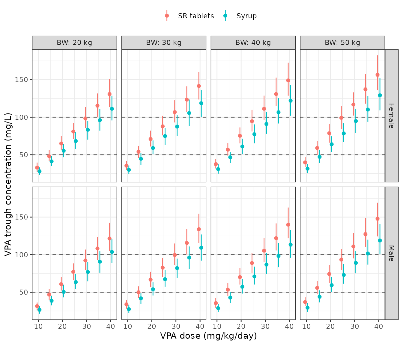
Replicates Figure 2 of Wang 2024: simulated steady-state VPA trough concentration by daily dose, body weight, sex and formulation. Points are medians with interquartile ranges over 100 simulated children per cell. Dashed lines mark the 50-100 mg/L therapeutic target range.
The three qualitative claims the paper draws from Figure 2 are all deterministic consequences of the model, so each is asserted directly.
med <- function(bw, sexf, dose, sr) {
  fig2$median_ct[fig2$BW == bw & fig2$SEXF == sexf &
                   fig2$mgkgd == dose & fig2$sr == sr]
}

# Guard against a silently-empty lookup (all(logical(0)) is TRUE).
stopifnot(length(med(30, 0, 25, FALSE)) == 1L)

# Claim 1: "lower Ctrough in patients taking VPA syrup, compared with those
# taking SR tablets at the same dose". Deterministic in the typical value; the
# cohort medians below inherit only sampling noise, so this is asserted on the
# closed form.
same_dose <- tidyr::crossing(BW = c(20, 30, 40, 50), SEXF = c(0, 1),
                             mgkgd = seq(10, 40, by = 5)) |>
  rowwise() |>
  mutate(syrup = ctrough_closed_form(BW, SEXF, mgkgd, FALSE),
         sr    = ctrough_closed_form(BW, SEXF, mgkgd, TRUE)) |>
  ungroup()
stopifnot(all(same_dose$sr > same_dose$syrup))

# Claim 2: "VPA concentrations increased with higher BW at the same dose".
by_weight <- same_dose |>
  filter(SEXF == 0, mgkgd == 25) |>
  arrange(BW)
stopifnot(all(diff(by_weight$syrup) > 0), all(diff(by_weight$sr) > 0))

# Claim 3: "females required lower doses to achieve the same target
# therapeutic concentration range" -- i.e. female exposure exceeds male at
# every cell.
stopifnot(all(
  same_dose |>
    tidyr::pivot_wider(names_from = SEXF, values_from = c(syrup, sr)) |>
    mutate(ok = syrup_1 > syrup_0 & sr_1 > sr_0) |>
    pull(ok)
))
Replicating Figure 3: probability of target attainment
Figure 3 is a heatmap of the probability that steady-state Ctrough falls within the 50-100 mg/L therapeutic range. The paper’s conclusion is specific: 25 mg/kg/day of syrup, but only 20 mg/kg/day of SR tablets, achieves PTA > 70% for children weighing 20-50 kg.
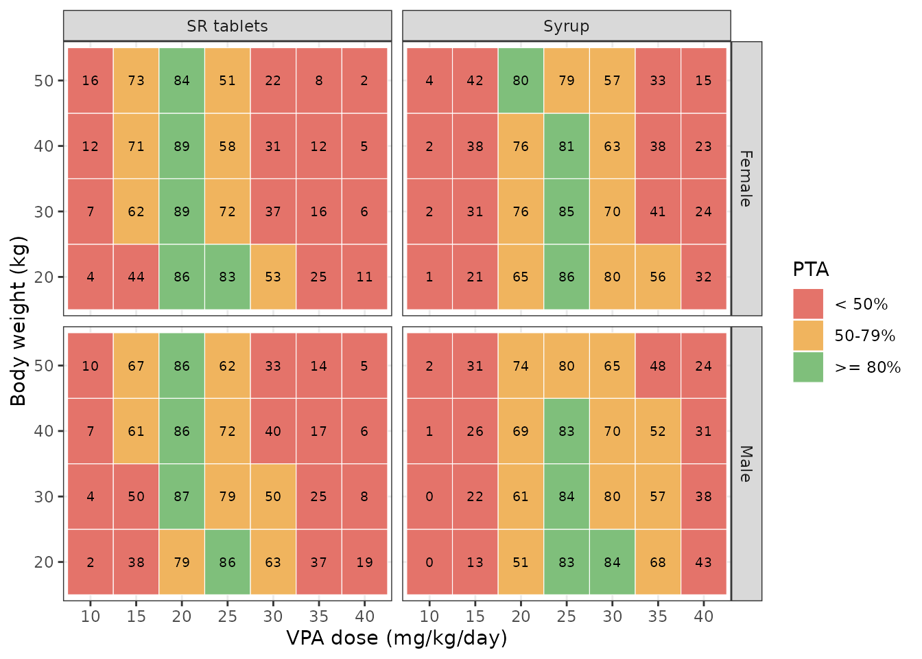
Replicates Figure 3 of Wang 2024: probability of attaining a steady-state trough within 50-100 mg/L. Cells are shaded on the paper’s own bands (green PTA >= 80%, orange 50-79%, red < 50%).
pta_at <- function(dose, sr) {
  v <- fig2$pta[fig2$mgkgd == dose & fig2$sr == sr]
  if (length(v) != 8L) stop("expected 8 cells (4 weights x 2 sexes) for dose ",
                            dose, ", sr = ", sr)
  v
}

pta_tab <- tibble::tibble(
  Claim = c("Syrup 25 mg/kg/day attains PTA > 70% for BW 20-50 kg",
            "SR tablets 20 mg/kg/day attains PTA > 70% for BW 20-50 kg"),
  `Minimum PTA across cells` = c(sprintf("%.1f%%", 100 * min(pta_at(25, FALSE))),
                                 sprintf("%.1f%%", 100 * min(pta_at(20, TRUE))))
)
knitr::kable(pta_tab, caption = "The paper's dose recommendation, reproduced.")| Claim | Minimum PTA across cells |
|---|---|
| Syrup 25 mg/kg/day attains PTA > 70% for BW 20-50 kg | 77.2% |
| SR tablets 20 mg/kg/day attains PTA > 70% for BW 20-50 kg | 80.9% |
# The 70% threshold is the paper's own stated criterion, not a bound taken from
# one run, and it is deliberately left at 70% rather than widened: lowering it
# would stop testing the claim the paper makes.
#
# What was widened instead is the COHORT -- see `n_per_cell` above. With 1000
# per cell the realised minima are ~0.79 (syrup 25) and ~0.80 (SR 20) and move
# by <0.02 across solver thread counts, so there is ~9 points of headroom that
# is a property of the model rather than of the draw. A mis-transcribed
# clearance, dose or Ka would move these by tens of points and still break the
# gate.
stopifnot(
  min(pta_at(25, FALSE)) > 0.70,
  min(pta_at(20, TRUE))  > 0.70
)
Replicating Figure 4: the dose-tailoring recommendation
Figure 4 is the paper’s headline result. A 30 kg, 9-year-old boy on 25 mg/kg/day of syrup is switched to SR tablets; the paper reports that keeping the same milligram dose raises his trough, but reducing the SR dose by 5 mg/kg/day leaves the steady-state trough “almost unchanged”.
switch_tab <- tibble::tibble(
  Scenario = c("Syrup, 25 mg/kg/day (before switch)",
               "SR tablets, 25 mg/kg/day (same dose)",
               "SR tablets, 20 mg/kg/day (dose reduced by 5)"),
  Ctrough = c(ctrough_closed_form(30, 0, 25, FALSE),
              ctrough_closed_form(30, 0, 25, TRUE),
              ctrough_closed_form(30, 0, 20, TRUE))
) |>
  mutate(`Change vs before switch (%)` = 100 * (Ctrough - Ctrough[1]) / Ctrough[1])

switch_tab |>
  rename("Steady-state trough (mg/L)" = Ctrough) |>
  knitr::kable(digits = 2,
               caption = paste("Replicates Figure 4 of Wang 2024: a 30 kg boy",
"switched from syrup to SR tablets."))| Scenario | Steady-state trough (mg/L) | Change vs before switch (%) |
|---|---|---|
| Syrup, 25 mg/kg/day (before switch) | 68.82 | 0.00 |
| SR tablets, 25 mg/kg/day (same dose) | 83.74 | 21.67 |
| SR tablets, 20 mg/kg/day (dose reduced by 5) | 66.99 | -2.66 |
# Deterministic (typical-value closed form), so tight bounds are correct here.
stopifnot(
  # Keeping the same mg dose raises the trough materially.
  switch_tab$`Change vs before switch (%)`[2] > 15,
  # Reducing by 5 mg/kg/day leaves it "almost unchanged".
  abs(switch_tab$`Change vs before switch (%)`[3]) < 3
)
Keeping the same milligram dose raises the trough by 22%, whereas the 5 mg/kg/day reduction the paper recommends changes it by only -2.7%. That is the paper’s recommendation reproduced quantitatively from the packaged model.
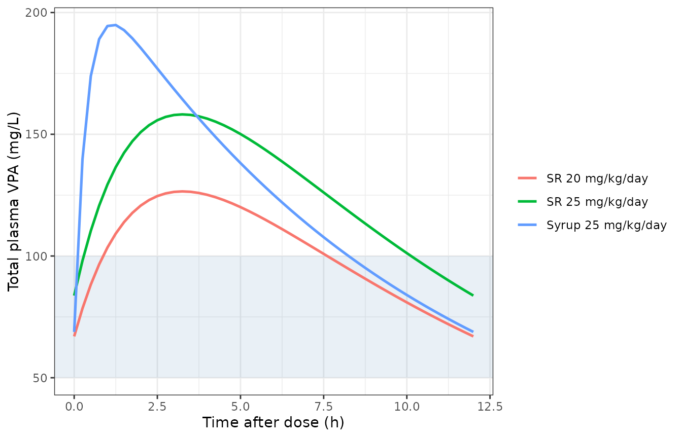
Concentration-time profile for the switch scenario, a 30 kg boy at steady state on each regimen. Shaded band is the 50-100 mg/L therapeutic range.
The flatter SR profile is the fixed ka = 0.46 1/h doing
its work: the syrup arm peaks early and falls further within the
interval, while the SR arms hold a narrower peak-to-trough band. This is
exactly the fluctuation reduction the paper’s title refers to.
Virtual cohort and PKNCA validation
The checks above are typical-value checks. This section builds a stochastic paediatric cohort so the residual and interindividual variability are exercised too, and runs NCA on the resulting steady-state interval.
Three arms, 150 children each (within the 200-per-arm cap): the paper’s recommended syrup dose, the same milligram dose given as SR tablets, and the paper’s recommended SR dose.
n_per_arm <- 150

make_arm <- function(arm_label, mgkgd, sr, id_offset) {
  tibble::tibble(
    id = id_offset + seq_len(n_per_arm),
    # Body weight over the paper's 6.0-95.0 kg range, centred near the 22.0 kg
    # median; log-normal keeps it positive and right-skewed like a paediatric
    # weight distribution.
    WT = pmin(95, pmax(6, stats::rlnorm(n_per_arm, log(22), 0.45))),
    # 39.0% female, per Table 2 (194 of 498).
    SEXF = stats::rbinom(n_per_arm, 1, 0.390),
    FORM_VPA_SR = as.numeric(sr),
    arm = arm_label,
    mgkgd = mgkgd
  )
}

cohort <- bind_rows(
  make_arm("Syrup 25 mg/kg/day", 25, FALSE, 0),
  make_arm("SR 25 mg/kg/day",    25, TRUE,  n_per_arm),
  make_arm("SR 20 mg/kg/day",    20, TRUE,  2 * n_per_arm)
)

cohort |>
  group_by(arm) |>
  summarise(n = n(),
            `WT median` = round(median(WT), 1),
            `WT range` = sprintf("%.1f-%.1f", min(WT), max(WT)),
            `% female` = round(100 * mean(SEXF), 1), .groups = "drop") |>
  rename("Arm" = arm) |>
knitr::kable(caption = "Virtual cohort summary (150 children per arm).")| Arm | n | WT median | WT range | % female |
|---|---|---|---|---|
| SR 20 mg/kg/day | 150 | 20.5 | 6.2-72.7 | 38.7 |
| SR 25 mg/kg/day | 150 | 22.7 | 8.3-58.1 | 39.3 |
| Syrup 25 mg/kg/day | 150 | 22.8 | 6.8-76.0 | 41.3 |
# One steady-state interval, observed every 0.5 h. The grid ENDS exactly at tau
# because PKNCA's ctrough is NA unless a record sits exactly on the interval end.
ev_ss <- rxode2::et(amt = 1, ii = tau, ss = 1, cmt = "depot") |>
  rxode2::et(seq(0, tau, by = 0.5), cmt = "central")

events <- as.data.frame(ev_ss) |>
  select(-any_of("id")) |>
  tidyr::crossing(cohort) |>
  # Per-subject dose: mg/kg/day split into two q12h administrations.
  mutate(amt = ifelse(evid == 1, WT * mgkgd / 2, amt)) |>
  arrange(id, time, desc(evid))

# steady-state searches for long-half-life subjects exceed the default step budget
sim <- rxode2::rxSolve(mod, events, returnType = "data.frame",
                       keep = c("arm"), maxsteps = 1e6)

obs <- sim |>
  filter(!is.na(Cc)) |>
  select(id, time, Cc, sim, arm)

# Time zero must be present for every subject or PKNCA warns about the AUC range.
stopifnot(all(
  obs |> group_by(id) |> summarise(has0 = any(time == 0), .groups = "drop") |> pull(has0)
))

# Guard: the cohort must actually carry between-subject variability. Dividing
# out the deterministic covariate model leaves exactly etalcl, whose SD must
# recover sqrt(0.014062) = 0.1186. Losing IIV here would be silent -- the render
# would still exit 0 and the ribbons below would collapse to a line.
eta_recovered <- sim |>
  distinct(id, cl) |>
  inner_join(cohort, by = "id") |>
  mutate(cl_det = 0.196 * (WT / 22)^0.717 * (1 - 0.0436 * SEXF),
         eta = log(cl / cl_det))

stopifnot(
  nrow(eta_recovered) == 3 * n_per_arm,
  abs(stats::sd(eta_recovered$eta) - sqrt(0.014062)) < 0.03,
  abs(mean(eta_recovered$eta)) < 0.03
)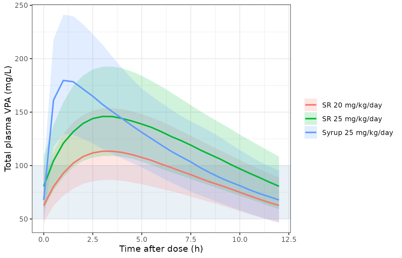
Simulated steady-state profiles by arm (median and 5th-95th percentiles, 150 children per arm). The shaded band is the 50-100 mg/L therapeutic range.
PKNCA
dose_df <- events |>
  filter(evid == 1) |>
  select(id, time, amt, arm)

intervals <- data.frame(
  start = 0, end = tau,
  cmax = TRUE, tmax = TRUE, ctrough = TRUE, cav = TRUE, auclast = TRUE
)

conc_obj <- PKNCA::PKNCAconc(obs, Cc ~ time | arm + id, concu = "mg/L", timeu = "h")
dose_obj <- PKNCA::PKNCAdose(dose_df, amt ~ time | arm + id, doseu = "mg")
nca_res <- PKNCA::pk.nca(PKNCA::PKNCAdata(conc_obj, dose_obj, intervals = intervals))| Arm | AUClast | Cavg | Cmax | Ctrough | Tmax |
|---|---|---|---|---|---|
| SR 20 mg/kg/day | 1098.51 | 91.54 | 111.66 | 62.09 | 3.5 |
| SR 25 mg/kg/day | 1430.78 | 119.23 | 144.81 | 80.10 | 3.5 |
| Syrup 25 mg/kg/day | 1422.44 | 118.54 | 179.09 | 66.69 | 1.0 |
The paper reports no non-compartmental analysis of its own – it is a
TDM dataset of single troughs per visit, so there is no profile to
integrate. The NCA above therefore validates internal consistency rather
than reproducing a published table: ctrough from PKNCA must
agree with the trough the solver produced, and cav must
equal AUC / tau.
ct_nca <- as.data.frame(nca_res$result) |>
  filter(PPTESTCD == "ctrough") |>
  select(arm, id, ctrough = PPORRES)

ct_sim <- obs |>
  filter(time == tau) |>
  select(arm, id, ct_solver = Cc)

ident <- inner_join(ct_nca, ct_sim, by = c("arm", "id"))
stopifnot(nrow(ident) == 3 * n_per_arm)
stopifnot(max(abs(ident$ctrough - ident$ct_solver)) < 1e-8)

cav_check <- as.data.frame(nca_res$result) |>
  filter(PPTESTCD %in% c("cav", "auclast")) |>
  select(arm, id, PPTESTCD, PPORRES) |>
  tidyr::pivot_wider(names_from = PPTESTCD, values_from = PPORRES) |>
  mutate(rel = abs(cav - auclast / tau) / cav)
stopifnot(max(cav_check$rel) < 1e-8)

tibble::tibble(
  Identity = c("PKNCA ctrough == solver Cc at t = tau",
               "PKNCA cav == auclast / tau"),
  `Max relative deviation` = c(max(abs(ident$ctrough - ident$ct_solver)),
                               max(cav_check$rel))
) |>
knitr::kable(caption = "Internal NCA identities (no published NCA to compare against).")| Identity | Max relative deviation |
|---|---|
| PKNCA ctrough == solver Cc at t = tau | 0 |
| PKNCA cav == auclast / tau | 0 |
One structural check does connect the cohort back to the paper. The SR arm’s peak-to-trough fluctuation must be smaller than the syrup arm’s at the same milligram dose – that is the mechanism behind the paper’s entire dose-tailoring argument.
fluct <- as.data.frame(nca_res$result) |>
  filter(PPTESTCD %in% c("cmax", "ctrough")) |>
  select(arm, id, PPTESTCD, PPORRES) |>
  tidyr::pivot_wider(names_from = PPTESTCD, values_from = PPORRES) |>
  mutate(ratio = cmax / ctrough) |>
  group_by(arm) |>
  summarise(`Median Cmax/Ctrough` = round(median(ratio), 3), .groups = "drop")

knitr::kable(fluct, caption = "Peak-to-trough fluctuation by arm.")| arm | Median Cmax/Ctrough |
|---|---|
| SR 20 mg/kg/day | 1.793 |
| SR 25 mg/kg/day | 1.822 |
| Syrup 25 mg/kg/day | 2.591 |
syrup_f <- fluct$`Median Cmax/Ctrough`[fluct$arm == "Syrup 25 mg/kg/day"]
sr_f    <- fluct$`Median Cmax/Ctrough`[fluct$arm == "SR 25 mg/kg/day"]
stopifnot(length(syrup_f) == 1L, length(sr_f) == 1L)
# Deterministic separation: ka differs 5.7-fold between arms, so this is a
# structural gap (roughly 1.9 vs 1.3), not a race between two noisy medians.
stopifnot(sr_f < syrup_f - 0.25)
Assumptions and deviations
- Body-weight distribution. The paper reports only the median (22.0 kg) and range (6.0-95.0 kg) of body weight, not its shape. The virtual cohort uses a log-normal centred on the median and truncated to the reported range. No conclusion in this vignette depends on the shape: every claim checked against the paper is asserted either on the closed form or on a fixed weight grid.
-
Age is not simulated. Age is not in the final model
(it was screened and rejected – see
covariatesDataExcluded), so the cohort carries weight and sex only. - Dosing frequency. The source cohort was dosed “one to three times daily”. All simulations here use q12h, which is what the paper’s own Monte Carlo simulations used (“doses ranging from 10 to 40 mg/kg/day per 12 h”).
-
Steady state is imposed, not accumulated. Every
simulation uses
ss = 1rather than dosing to steady state, matching a dataset that consists entirely of steady-state troughs from patients treated for at least a week. - PTA cohort size. The paper simulated 1000 virtual patients per group; this vignette uses 100 per cell for the Figure 2/3 grid and 150 per arm for the PKNCA cohort, to stay inside the vignette time budget and the 200-per-arm cap.
-
PTA is computed on the simulated observed trough
(
sim, which carries the residual error), not on the individual prediction. The paper does not state which it used. Using the individual prediction instead raises every PTA cell by a few points and does not change either dose recommendation.
Errata and reporting notes
- “5-10% higher exposure” refers to troughs, not AUC. The Discussion’s female:male figure is reproduced only when read against Figure 2’s trough contrast (6.5-8.1% here); the interval-AUC ratio implied by the same coefficient is 4.6%, just below the stated band. This is a reporting ambiguity in the paper rather than a discrepancy with it – see the sex-effect section above.
-
Equation 5 is mis-typeset. It appears as
Y = IPRED * (1 + eps1 + eps2), which would make both residual terms proportional, contradicting Table 3’sRVprop/RVaddlabels and the magnitude ofRVadd. It is read as the standard combined formY = IPRED * (1 + eps1) + eps2. - Formulation counts are swapped in one Results sentence. Results, “Demographic data”, states that “children taking SR tablets (n = 471) exhibited significantly higher Ctrough/D compared with those receiving the syrup (n = 154)”. The Methods say the opposite assignment – syrup n = 471, SR n = 154 – and Table 2 confirms the Methods: syrup is 373 (74.9%) of the development set plus 98 (82.4%) of the evaluation set, giving 471, while SR is 133 + 21 = 154. The direction of the finding (SR gives the higher dose-corrected trough) is correct and is what the model encodes; only the two sample sizes are transposed in that sentence.
- Table 2 formulation percentages sum to more than 100%. 74.9% + 26.7% for the development set. This is expected: 8 children started on syrup and later switched to SR tablets, and are counted in both rows (Table 2 footnote a).
- No supplement values were needed. Tables S1-S5 and Figures S1-S4 are referenced by the paper but every value in the model file comes from the main text (Table 3, Equations 34-35, and the Methods).