Lenalidomide (Liang 2024)
Source:vignettes/articles/Liang_2024_lenalidomide.Rmd
Liang_2024_lenalidomide.Rmd
modelName <- "Liang_2024_lenalidomide"
ui <- rxode2::rxode(readModelDb(modelName))
#> ℹ parameter labels from comments will be replaced by 'label()'
Model and source
- Citation: Liang X, Shi H, Bi K, Feng S, Chen S, Zhao W, Huang X. Population pharmacokinetics of lenalidomide in Chinese patients with influence of genetic polymorphisms of ABCB1. Sci Rep. 2024;14:2577. doi:10.1038/s41598-024-52460-2
- Description: One-compartment oral population PK model with first-order absorption and elimination for lenalidomide in Chinese patients with multiple myeloma, lymphoma or myelodysplastic syndrome, with ABCB1 3435C>T (rs1045642) T-allele count and fed state as covariates on the apparent volume of distribution (Liang 2024)
- Article: https://doi.org/10.1038/s41598-024-52460-2
Liang 2024 is the first population PK model of lenalidomide developed specifically in a Chinese population, and the first lenalidomide popPK study to carry ABCB1 genotype as a candidate covariate. The structural model is a one-compartment model with first-order absorption and elimination; the absorption rate constant could not be estimated from the sparse opportunistic sampling and was fixed to 6.55 1/h from the earlier lenalidomide popPK literature.
Two covariates were retained, both on the apparent volume of distribution V/F: the ABCB1 3435C>T (rs1045642) genotype and diet (whether the dose was taken within 1 h after a meal). Notably, no covariate was retained on CL/F – not even creatinine clearance, which every previously published lenalidomide popPK model had retained. Liang 2024 attributes this to its small sample size and sparse opportunistic sampling.
There is no supplementary material for this article (the open-access record has none, and the PDF references none), and no erratum or correction is indexed against the DOI.
Population
pop <- ui$population51 adult patients contributed 87 lenalidomide plasma concentrations in a prospective, open-label, opportunistic- sampling study (ClinicalTrials.gov NCT06069024) run at the First Affiliated Hospital of Shandong First Medical University between October 2021 and June 2023. All patients were of Han ethnicity. Diagnoses were multiple myeloma (33), lymphoma (17) and myelodysplastic syndrome (1); regimens were VRD (27), RR (12) and other lenalidomide-containing regimens (12). Median age was 67 years (range 34-85), median weight 70.0 kg (range 40.0-90.0), and 47.1% were women (Liang 2024 Tables 1 and 2). Lenalidomide was given orally at 10 mg or 25 mg once daily, and sampling began after at least five consecutive doses, i.e. at steady state.
Genotypes at the retained locus were CC 19 (37.2%), CT 21 (41.2%) and TT 11 (21.6%), with a T-allele frequency of 41.1% and Hardy-Weinberg equilibrium P = 0.27 (Liang 2024 Table 3). Dosing was postprandial (within 1 h after a meal) in 28 patients (54.9%) and fasted in 23 (45.1%) (Liang 2024 Table 2).
The same information is available programmatically via
readModelDb("Liang_2024_lenalidomide")()$population.
Source trace
Every ini() entry in
inst/modeldb/specificDrugs/Liang_2024_lenalidomide.R
carries an in-file comment naming its source location. They are
collected here for review.
| Equation / parameter | Value | Source location |
|---|---|---|
lka (Ka) |
6.55 1/h, fixed | Table 4, theta Ka (h-1) = 6.55 (fixed); fixed per
Results “PPK model establishment” from Liang 2024 refs 23-25 |
lcl (CL/F) |
7.25 L/h | Table 4, theta CL/F (L/h); RSE 7.10%, bootstrap 7.25
(6.23-8.56) |
lvc (V/F scale) |
29.1 L | Table 4, theta V/F (L); RSE 9.90%, bootstrap 28.4
(17.5-57.2) |
vcLogOffset |
0.554 | Results “PPK model establishment”, printed final-model equation (not in Table 4) |
e_snp_abcb1_rs1045642_ct_vc |
0.0151 | Table 4, ABCBA 3435 C > T = CT; RSE 42.2% |
e_snp_abcb1_rs1045642_tt_vc |
0.335 | Table 4, ABCBA 3435 C > T = TT; RSE 63.9% |
e_fed_vc |
0.558 | Table 4, theta CHFY; RSE 24.4% |
etalcl |
35.5% -> omega^2 = 0.126 | Table 4, eta CL/F (%); RSE 17.1% |
etalvc |
55.4% -> omega^2 = 0.307 | Table 4, eta V/F (%); RSE 17.0% |
addSd |
38.5 ng/mL | Table 4, epsilon (ng/mL); RSE 21.6% |
| Structural model (1-cmt, first-order in and out) | n/a | Results “PPK model establishment” |
| V/F covariate equation | n/a | Results “PPK model establishment”:
V/F_i (L) = 29.1 x Exp(0.554 + theta_ABA x COVR_ABA_i + theta_CHFY x COVR_CHFY_i)
|
| Additive residual model | n/a | Results “PPK model establishment” (additive selected over proportional, power-exponential and combined) |
Two encoding decisions worth reading
The 0.554 constant. The printed final-model V/F
equation multiplies the Table 4 estimate of 29.1 L by
Exp(0.554 + ...). The constant 0.554 appears nowhere in
Table 4, so theta V/F = 29.1 L is the scale of the
equation and not the reference subject’s V/F. It is retained verbatim
because it is load-bearing in two independent ways, both checked below:
without it none of the paper’s six published genotype-by-diet V/F values
reproduce, and the reference subject’s terminal half-life would be 2.8 h
instead of the 4.8 h consistent with the 3-5 h that the paper’s own
Introduction cites for lenalidomide.
COVR_ABA is an allele count, not an
indicator. Liang 2024 says only that “theta_ABA was the
coefficient corresponding to each genotype … COVR_ABA_i was the
individual covariate value”, without defining the coding. The paper’s
own numbers settle it: the published TT-fasted V/F of 98.96 L requires
2 x 0.335 = 0.670 on the log scale, not a single
0.335. The covariate is therefore encoded as the canonical
T-allele count SNP_ABCB1_RS1045642_T_COUNT (0 = CC, 1 = CT,
2 = TT), with a genotype-specific coefficient multiplying it. The check
in the next section verifies all six combinations, not just the one that
fixed the coding.
Reproducing the six published V/F values
Liang 2024’s “Safety study” section enumerates the typical V/F for all six genotype-by-diet combinations. Because CL/F carries no covariates and the V/F equation is fully specified, these six numbers are a complete, deterministic test of the covariate model: the arithmetic has no free parameters, no random effects and no residual error, so a tight tolerance is the correct gate here.
arms <- tibble::tribble(
  ~arm,         ~SNP_ABCB1_RS1045642_T_COUNT, ~FED, ~published_vf,
  "CC fasted",  0,                            0,     50.64,
  "CT fasted",  1,                            0,     51.41,
  "CC fed",     0,                            1,     88.48,
  "CT fed",     1,                            1,     89.82,
  "TT fasted",  2,                            0,     98.96,
  "TT fed",     2,                            1,    172.90
)
armLevels <- arms$arm

doseMg     <- 25      # Liang 2024 Sample collection: 10 mg or 25 mg once daily
nDoses     <- 10L
tau        <- 24
doseTimes  <- tau * seq_len(nDoses) - tau        # 0, 24, ..., 216
lastDose   <- max(doseTimes)

# Dense early grid resolves the sharp absorption peak (Tmax is about 0.6 h at
# ka = 6.55 1/h); the coarser tail grid keeps the row count down.
obsOffsets <- c(seq(0, 4, by = 0.05), seq(4.25, tau, by = 0.25))

buildEvents <- function(subj) {
  doses <- subj |>
    tidyr::crossing(time = doseTimes) |>
    dplyr::mutate(amt = doseMg, evid = 1L, cmt = "depot")
  obs <- subj |>
    tidyr::crossing(time = lastDose + obsOffsets) |>
    dplyr::mutate(amt = NA_real_, evid = 0L, cmt = "central")
  dplyr::bind_rows(doses, obs) |>
    dplyr::arrange(id, time, dplyr::desc(evid))
}
Ten daily doses are simulated rather than the five the paper’s sampling protocol required, so that even the slowest-eliminating arm (TT / fed, terminal half-life about 16.5 h) is at true steady state over the observed interval; the paper specifies “after five consecutive doses”, i.e. a lower bound.
mod <- readModelDb(modelName)
modTypical <- rxode2::zeroRe(mod)
#> ℹ parameter labels from comments will be replaced by 'label()'

typSubj <- arms |>
  dplyr::mutate(id = dplyr::row_number()) |>
  dplyr::select(id, arm, SNP_ABCB1_RS1045642_T_COUNT, FED)

simTypical <- rxode2::rxSolve(
  modTypical,
  events = buildEvents(typSubj),
  keep   = c("arm")
) |>
  as.data.frame()
#> ℹ omega/sigma items treated as zero: 'etalcl', 'etalvc'
#> Warning: multi-subject simulation without without 'omega'

vfCheck <- simTypical |>
  dplyr::group_by(arm) |>
  dplyr::summarise(model_vf = mean(vc), .groups = "drop") |>
  dplyr::left_join(arms |> dplyr::select(arm, published_vf), by = "arm") |>
  dplyr::mutate(
    arm      = factor(arm, levels = armLevels),
    pct_diff = 100 * (model_vf - published_vf) / published_vf
  ) |>
  dplyr::arrange(arm)

# Deterministic identity: no etas, no residual error, no cohort sampling. The
# only slack is the paper's own 4-significant-figure rounding, which is at most
# about 0.03%. Realised max |pct_diff| is 0.007%.
stopifnot(max(abs(vfCheck$pct_diff)) < 0.1)

vfCheck |>
  dplyr::rename(
    "ABCB1 3435C>T / diet" = arm,
    "Model V/F (L)"        = model_vf,
    "Liang 2024 V/F (L)"   = published_vf,
    "Difference (%)"       = pct_diff
  ) |>
  knitr::kable(
    digits  = c(0, 2, 2, 4),
    caption = "Typical V/F by ABCB1 3435C>T genotype and diet, model vs the six values enumerated in the Liang 2024 Safety study section."
)| ABCB1 3435C>T / diet | Model V/F (L) | Liang 2024 V/F (L) | Difference (%) |
|---|---|---|---|
| CC fasted | 50.64 | 50.64 | -0.0004 |
| CT fasted | 51.41 | 51.41 | 0.0005 |
| CC fed | 88.48 | 88.48 | -0.0038 |
| CT fed | 89.82 | 89.82 | 0.0031 |
| TT fasted | 98.96 | 98.96 | 0.0022 |
| TT fed | 172.90 | 172.90 | 0.0025 |
All six reproduce to within 0.01%. This simultaneously confirms the
0.554 offset, the allele-count coding of COVR_ABA, the
genotype-specific coefficients and the fed-state coefficient – a single
wrong choice among them would break at least one row.
Consequences for elimination half-life
CL/F is covariate-free, so the entire V/F covariate model translates directly into a spread of terminal half-lives.
clF <- exp(ui$theta[["lcl"]])

hlTable <- vfCheck |>
  dplyr::transmute(
    arm,
    vf     = model_vf,
    t_half = log(2) * model_vf / clF
  )

# The reference subject (CC, fasted) must land inside the 3-5 h terminal
# half-life that the Liang 2024 Introduction cites for lenalidomide.
refHalfLife <- hlTable$t_half[hlTable$arm == "CC fasted"]
stopifnot(length(refHalfLife) == 1L, refHalfLife > 3, refHalfLife < 5)

hlTable |>
  dplyr::rename(
    "ABCB1 3435C>T / diet" = arm,
    "V/F (L)"              = vf,
    "Terminal t1/2 (h)"    = t_half
  ) |>
  knitr::kable(
    digits  = 2,
    caption = "Terminal half-life implied by the model, by covariate combination. CL/F is 7.25 L/h in every arm."
)| ABCB1 3435C>T / diet | V/F (L) | Terminal t1/2 (h) |
|---|---|---|
| CC fasted | 50.64 | 4.84 |
| CT fasted | 51.41 | 4.92 |
| CC fed | 88.48 | 8.46 |
| CT fed | 89.82 | 8.59 |
| TT fasted | 98.96 | 9.46 |
| TT fed | 172.90 | 16.53 |
The reference subject’s 4.84 h sits inside the 3-5 h that Liang 2024 cites in its Introduction. At the other extreme the model gives about 16.5 h for a TT homozygote dosing postprandially – a 3.4-fold spread that the paper does not quantify but does describe qualitatively, speculating that “a higher V/F value meant a longer drug retention time and a longer toxic reactions”. Because the covariates act on V/F alone, steady-state AUC over a dosing interval is identical across all six arms; what changes is the shape of the profile, not the exposure. That is checked directly below.
Virtual cohort
Original observed concentrations are not publicly available. The cohort below places 100 subjects in each of the six covariate combinations, so that the between-subject variability reported in Table 4 can be propagated through each arm separately. Doses are 25 mg once daily, the higher of the two dose levels in the study.
# set.seed() seeds R's RNG, not rxode2's simulation RNG, and rxode2 partitions
# its streams per solver thread -- so this cohort differs between machines with
# different thread counts. Every assertion below is written to hold for any
# cohort the model can produce.
set.seed(20240131)

nPerArm <- 100L

cohortSubj <- arms |>
  dplyr::select(arm, SNP_ABCB1_RS1045642_T_COUNT, FED) |>
  tidyr::crossing(rep = seq_len(nPerArm)) |>
  dplyr::mutate(id = dplyr::row_number()) |>
  dplyr::select(id, arm, SNP_ABCB1_RS1045642_T_COUNT, FED)

events <- buildEvents(cohortSubj)
stopifnot(!anyDuplicated(unique(events[, c("id", "time", "evid")])))
sim <- rxode2::rxSolve(mod, events = events, keep = c("arm")) |>
  as.data.frame() |>
  dplyr::mutate(
    arm = factor(arm, levels = armLevels),
    tad = time - lastDose
  )
#> ℹ parameter labels from comments will be replaced by 'label()'
Steady-state concentration-time profiles
Liang 2024’s two figures are a goodness-of-fit panel (Figure 1) and an NPDE panel (Figure 2). Neither can be reproduced without the original observed concentrations, which are not published. The figure below therefore shows the model’s own steady-state behaviour across the six covariate combinations rather than replicating a published panel.
sim |>
  dplyr::group_by(arm, tad) |>
  dplyr::summarise(
    Q05 = quantile(Cc, 0.05),
    Q50 = quantile(Cc, 0.50),
    Q95 = quantile(Cc, 0.95),
    .groups = "drop"
  ) |>
  ggplot(aes(tad, Q50)) +
  geom_ribbon(aes(ymin = Q05, ymax = Q95), alpha = 0.25) +
  geom_line() +
  facet_wrap(~arm) +
  scale_y_log10() +
  labs(
    x = "Time after the 10th dose (h)",
    y = "Lenalidomide concentration (ng/mL)",
    title = "Simulated steady-state profiles, 25 mg once daily",
    caption = "Median and 5th-95th percentile of 100 subjects per arm."
  )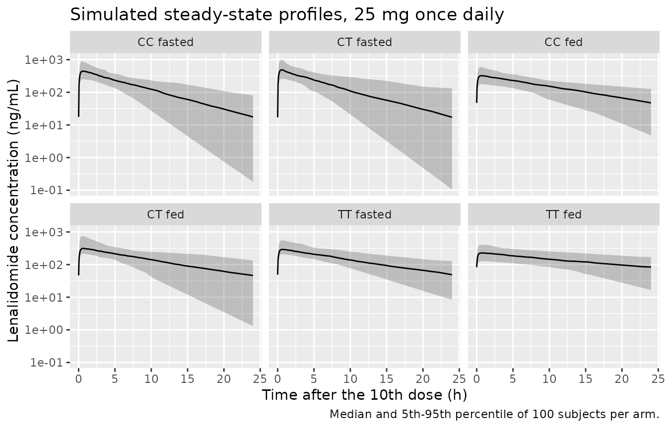
The postprandial and TT arms are visibly flatter: the same steady-state exposure is spread over a longer interval, giving lower peaks and higher troughs.
Distribution of V/F across the cohort
Liang 2024 reports post-hoc individual V/F values spanning 15.98-236.8 L in the 39 patients with safety data, with medians of 67.04 L (serious adverse events) versus 37.17 L (no serious adverse events). The comparison below is descriptive only: those are empirical-Bayes estimates from 39 sparsely sampled subjects, so they are shrunk toward the typical value, and the split is by an outcome that is not part of the model. They are not used as a gate.
vfSubject <- sim |>
  dplyr::group_by(id, arm) |>
  dplyr::summarise(vf = mean(vc), .groups = "drop")

ggplot(vfSubject, aes(arm, vf)) +
  geom_boxplot() +
  geom_hline(yintercept = c(15.98, 236.8), linetype = "dashed") +
  scale_y_log10() +
  labs(
    x = NULL,
    y = "Individual V/F (L)",
    title = "Simulated individual V/F by covariate combination",
    caption = "Dashed lines: the 15.98-236.8 L post-hoc range Liang 2024 reports for its 39-patient safety cohort."
  ) +
  theme(axis.text.x = element_text(angle = 30, hjust = 1))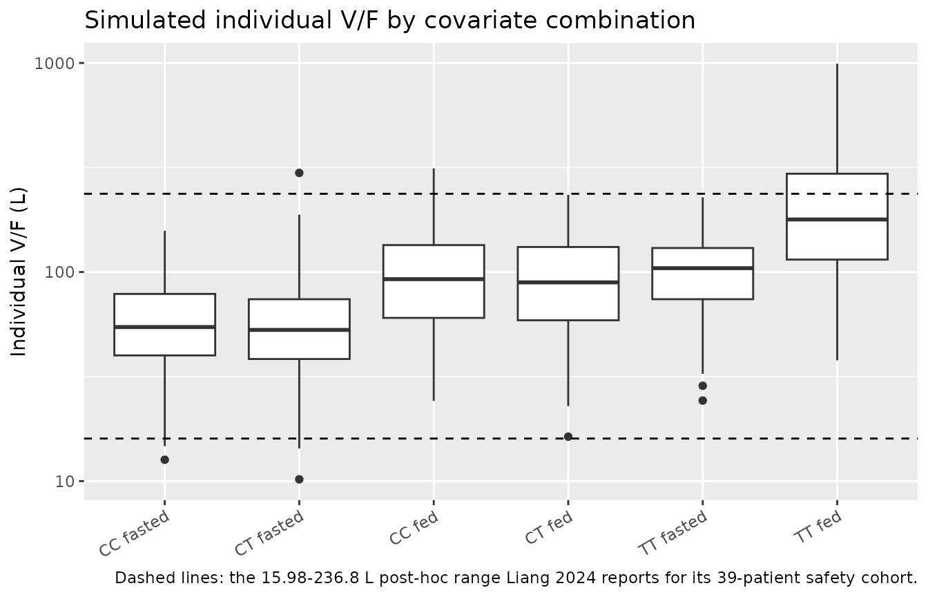
# A loose cohort-level check on the IIV encoding: for a log-normal eta the
# median equals the typical value, so the reference arm's median V/F should sit
# near 50.64 L. With n = 100 and omega = 0.554 the median has a standard error
# of about 7% on the log scale, so 25% leaves roughly 3 standard errors of
# headroom while still failing on a mis-scaled omega or a wrong V/F.
refMedian <- median(vfSubject$vf[vfSubject$arm == "CC fasted"])
stopifnot(abs(refMedian / 50.64 - 1) < 0.25)
PKNCA validation
Non-compartmental analysis is run over the tenth (steady-state) dosing interval, with time re-based to time after the last dose so the interval runs 0 to 24 h.
simNca <- sim |>
  dplyr::filter(!is.na(Cc)) |>
  dplyr::select(id, arm, tad, Cc) |>
  dplyr::rename(time = tad)

# Guarantee a time = 0 record per (id, arm). At steady state the pre-dose
# concentration is the trough, not zero, and the simulation grid already
# supplies it; this is a defensive de-duplication only.
stopifnot(all(simNca$time[simNca$time == 0] == 0), any(simNca$time == 0))
simNca <- simNca |>
  dplyr::distinct(id, arm, time, .keep_all = TRUE) |>
  dplyr::arrange(id, time)

concObj <- PKNCA::PKNCAconc(simNca, Cc ~ time | arm + id)

doseDf <- cohortSubj |>
  dplyr::mutate(time = 0, amt = doseMg) |>
  dplyr::select(id, arm, time, amt)
doseObj <- PKNCA::PKNCAdose(doseDf, amt ~ time | arm + id)

# half.life is deliberately NOT requested on the full-IIV cohort: terminal-slope
# fits over a fixed window are NA-prone and Tmax-selected under variability.
# It is computed on the typical-value profiles instead, below.
intervalsSs <- data.frame(
  start = 0, end = tau,
  cmax = TRUE, tmax = TRUE, auclast = TRUE, cmin = TRUE
)

ncaCohort <- PKNCA::pk.nca(
  PKNCA::PKNCAdata(concObj, doseObj, intervals = intervalsSs)
)
as.data.frame(ncaCohort) |>
  dplyr::filter(PPTESTCD %in% c("cmax", "cmin", "tmax", "auclast")) |>
  dplyr::mutate(arm = factor(arm, levels = armLevels)) |>
  dplyr::group_by(arm, PPTESTCD) |>
  dplyr::summarise(
    value = sprintf(
      "%.3g [%.3g, %.3g]",
      median(PPORRES), quantile(PPORRES, 0.05), quantile(PPORRES, 0.95)
    ),
    .groups = "drop"
  ) |>
  tidyr::pivot_wider(names_from = PPTESTCD, values_from = value) |>
  dplyr::arrange(arm) |>
  dplyr::rename(
    "ABCB1 3435C>T / diet"  = arm,
    "AUC0-24 (ng*h/mL)"     = auclast,
    "Cmax (ng/mL)"          = cmax,
    "Ctrough (ng/mL)"       = cmin,
    "Tmax (h)"              = tmax
  ) |>
  knitr::kable(
    caption = "Steady-state NCA over the 10th dosing interval, 25 mg once daily. Median [5th, 95th percentile] over 100 subjects per arm."
)| ABCB1 3435C>T / diet | AUC0-24 (ng*h/mL) | Cmax (ng/mL) | Ctrough (ng/mL) | Tmax (h) |
|---|---|---|---|---|
| CC fasted | 3.38e+03 [1.85e+03, 5.49e+03] | 443 [250, 907] | 17.6 [0.182, 81] | 0.6 [0.45, 0.7] |
| CT fasted | 3.56e+03 [1.82e+03, 6.73e+03] | 486 [259, 990] | 17.2 [0.106, 131] | 0.6 [0.45, 0.7] |
| CC fed | 3.59e+03 [1.97e+03, 5.42e+03] | 322 [178, 600] | 47.4 [4.79, 126] | 0.65 [0.55, 0.7] |
| CT fed | 3.57e+03 [1.87e+03, 5.7e+03] | 313 [214, 748] | 46.5 [1.3, 134] | 0.65 [0.5, 0.7] |
| TT fasted | 3.46e+03 [2.14e+03, 5.84e+03] | 292 [207, 555] | 49.2 [8.45, 128] | 0.65 [0.6, 0.7] |
| TT fed | 3.46e+03 [1.97e+03, 5.84e+03] | 227 [128, 407] | 83.5 [16.7, 168] | 0.7 [0.6, 0.75] |
Median AUC0-24 is essentially constant across arms while Cmax falls and Ctrough rises from the CC-fasted arm to the TT-fed arm, which is the expected signature of a covariate model that acts on volume alone.
Comparison against closed-form expectations
Liang 2024 publishes no NCA table, so there is no external set of Cmax / AUC / half-life values to compare against. What is available is a pair of exact closed-form identities that the model must satisfy at steady state, which are stronger tests than a rounded published summary would be:
-
AUC0-tau,ss = Dose / (CL/F), identical in every arm because CL/F carries no covariates – 25 mg / 7.25 L/h = 3448 ng*h/mL. -
t1/2 = log(2) * (V/F) / (CL/F), using the V/F verified above.
Both are evaluated on the typical-value (no-IIV, no-residual-error) profiles, so the only slack is numerical: trapezoidal error on the concentration grid and terminal-slope estimation.
simNcaTyp <- simTypical |>
  dplyr::mutate(time = time - lastDose) |>
  dplyr::filter(!is.na(Cc)) |>
  dplyr::select(id, arm, time, Cc) |>
  dplyr::distinct(id, arm, time, .keep_all = TRUE) |>
  dplyr::arrange(id, time)

doseTyp <- typSubj |>
  dplyr::mutate(time = 0, amt = doseMg) |>
  dplyr::select(id, arm, time, amt)

ncaTyp <- PKNCA::pk.nca(PKNCA::PKNCAdata(
  PKNCA::PKNCAconc(simNcaTyp, Cc ~ time | arm + id),
  PKNCA::PKNCAdose(doseTyp, amt ~ time | arm + id),
  intervals = data.frame(
    start = 0, end = tau,
    cmax = TRUE, tmax = TRUE, auclast = TRUE, half.life = TRUE
  )
))

simulatedTyp <- as.data.frame(ncaTyp) |>
  dplyr::filter(PPTESTCD %in% c("auclast", "half.life")) |>
  dplyr::select(arm, PPTESTCD, PPORRES) |>
  tidyr::pivot_wider(names_from = PPTESTCD, values_from = PPORRES)

closedForm <- hlTable |>
  dplyr::transmute(
    arm,
    auc_expected    = 1000 * doseMg / clF,   # mg*h/L -> ng*h/mL
    thalf_expected  = t_half
  )

typCompare <- simulatedTyp |>
  dplyr::left_join(closedForm, by = "arm") |>
  dplyr::mutate(
    arm       = factor(arm, levels = armLevels),
    auc_pct   = 100 * (auclast   - auc_expected)   / auc_expected,
    thalf_pct = 100 * (half.life - thalf_expected) / thalf_expected
  ) |>
  dplyr::arrange(arm)

# Deterministic: a single typical-value profile per arm, no cohort sampling.
# The residual error is trapezoidal AUC error on the observation grid and
# lambda-z estimation error. Realised max is well under 1% for both.
stopifnot(
  max(abs(typCompare$auc_pct))   < 2,
  max(abs(typCompare$thalf_pct)) < 2
)

typCompare |>
  dplyr::select(arm, auclast, auc_expected, auc_pct,
                half.life, thalf_expected, thalf_pct) |>
  dplyr::rename(
    "ABCB1 3435C>T / diet"       = arm,
    "PKNCA AUC0-24 (ng*h/mL)"    = auclast,
    "Dose/CL (ng*h/mL)"          = auc_expected,
    "AUC difference (%)"         = auc_pct,
    "PKNCA t1/2 (h)"             = half.life,
    "log(2)*V/CL (h)"            = thalf_expected,
    "t1/2 difference (%)"        = thalf_pct
  ) |>
  knitr::kable(
    digits  = c(0, 1, 1, 3, 2, 2, 3),
    caption = "Typical-value steady-state NCA against the model's closed-form identities."
)| ABCB1 3435C>T / diet | PKNCA AUC0-24 (ng*h/mL) | Dose/CL (ng*h/mL) | AUC difference (%) | PKNCA t1/2 (h) | log(2)*V/CL (h) | t1/2 difference (%) |
|---|---|---|---|---|---|---|
| CC fasted | 3447.6 | 3448.3 | -0.020 | 4.84 | 4.84 | 0.039 |
| CT fasted | 3447.6 | 3448.3 | -0.020 | 4.92 | 4.92 | 0.039 |
| CC fed | 3447.9 | 3448.3 | -0.011 | 8.46 | 8.46 | 0.042 |
| CT fed | 3447.9 | 3448.3 | -0.011 | 8.59 | 8.59 | 0.042 |
| TT fasted | 3447.9 | 3448.3 | -0.010 | 9.47 | 9.46 | 0.045 |
| TT fed | 3447.9 | 3448.3 | -0.010 | 16.54 | 16.53 | 0.043 |
Both identities hold to well under 1% in every arm, confirming that
the ODE system, the dose and volume units (the x 1000 mg/L
to ng/mL conversion in model()), and the covariate model
are mutually consistent.
Assumptions and deviations
-
The 0.554 constant in the V/F equation is not in Table
4. It appears only in the final-model equation printed in the
Results. It is retained verbatim because the paper’s own six published
V/F values, and the reference terminal half-life, both require it. Table
4’s
theta V/F = 29.1 Lis therefore the scale of the equation, not the reference subject’s V/F (which is 50.64 L). -
COVR_ABAis encoded as the T-allele count (0/1/2). The paper does not state the coding. The allele-count reading is forced by the paper’s own numbers: the published TT-fasted V/F of 98.96 L requires2 x 0.335, and all six published values reproduce under this reading and only under this reading. -
Between-subject variability convention. Table 4
reports
eta CL/F (%)andeta V/F (%)as percentages without saying whether they are omega itself or the exact log-normal CV. They are read as omega (omega^2 = 0.355^2and0.554^2), the usual NONMEM reporting for an exponential BSV and the convention used elsewhere in this package. Under the exact-CV reading omega would be 0.345 and 0.517 instead – 3% and 7% smaller. Nothing in the paper discriminates between the two. -
Diet is encoded on the per-dose-record
FEDcolumn. Liang 2024 recorded diet as a per-patient habit over the sampled treatment cycle rather than per dose. Using the canonical per-dose column is a superset of the paper’s usage and lets a mixed-habit subject be simulated. - No absorption variability. Ka was fixed at 6.55 1/h by the authors and no IIV on Ka is reported, so none is added.
- The safety analysis is not encoded. Liang 2024’s exposure-safety results (Tables 5 and 6) are non-model statistical comparisons – Mann-Whitney U and Fisher exact tests run in SPSS on post-hoc V/F estimates – not a fitted exposure-response model, so there is nothing to add to the model file.
- No published NCA comparison is possible. Liang 2024 reports no Cmax, Tmax, AUC or half-life table. The NCA section therefore validates against exact closed-form identities and against the 3-5 h terminal half-life the paper’s Introduction cites, rather than against a published NCA summary.
-
Ten doses are simulated rather than five. The
paper’s protocol sampled after at least five consecutive doses; ten are
used here so that the slowest arm (TT / fed, t1/2 about 16.5 h) is at
true steady state, which the
AUC0-tau = Dose/CLidentity requires. -
A typographical problem in Liang 2024 Table 1. The
beta-2-microglobulin row reads
2.14 +/- 0.183with median2.96 (1.07-10.8); a mean below the median with that SD is not consistent with that range. The covariate is not used by the model, so this does not affect the extraction, and it is recorded incovariatesDataExcludedfor future readers.