Oxcarbazepine and its 10-monohydroxy derivative in children with obesity (Sinha 2026)
Source:vignettes/articles/Sinha_2026_oxcarbazepine.Rmd
Sinha_2026_oxcarbazepine.RmdModel and source
#> ℹ parameter labels from comments will be replaced by 'label()'- Citation: Sinha J, Zimmerman K, Balevic SJ, Hornik C, Muller WJ, Rathore M, Meyer M, Finkelstein Y, Al-Uzri A, Lakhotia A, Goldstein S, Chen JY, Anand R, Gonzalez D. Population Pharmacokinetic Modeling of Oxcarbazepine and Its Active Metabolite 10-Monohydroxy Derivative to Inform Dosing in Children with Obesity. Clin Pharmacokinet. 2026;65:329-344. doi:10.1007/s40262-025-01579-0. Correction: Clin Pharmacokinet. 2026;65:345. doi:10.1007/s40262-025-01613-1 (Eq. 10 was printed as TV_V,MHD = 50(PKWT/50)^0.752 but should read TV_V,OXZ = 33.1(PKWT/50)^0.752; no parameter value changed).
- Description: Joint parent-metabolite population PK model for oral oxcarbazepine (OXZ) and its active 10-monohydroxy derivative (MHD) in children with and without obesity, aged 44 days to 20.9 years (Sinha 2026). One-compartment OXZ plus one-compartment MHD with first-order absorption, complete conversion of OXZ to MHD (the OXZ elimination clearance IS the MHD formation clearance), molar-mass-corrected bidirectional mass transfer, and a first-order MHD-to-OXZ back-transformation. All clearances and volumes are allometrically scaled to pharmacokinetic weight (PKWT), a fat-free-mass-based body-size descriptor, referenced to 50 kg; body size was the only covariate retained.
- Article: https://doi.org/10.1007/s40262-025-01579-0
Oxcarbazepine (OXZ) is an antiepileptic whose pharmacological activity is carried almost entirely by its active metabolite, the 10-monohydroxy derivative (MHD). OXZ is cleared extremely fast (~175 L/h in healthy adults) by ubiquitously expressed cytosolic aldo-keto reductases, essentially all of it via conversion to MHD; MHD is then cleared slowly (~3 L/h). The result is a roughly 45-fold higher plasma exposure of MHD than of parent OXZ after an oral OXZ dose.
The packaged model is Sinha 2026’s final model M6: a one-compartment OXZ compartment with first-order absorption feeding a one-compartment MHD, with
- complete conversion – OXZ’s elimination clearance is MHD’s formation clearance, so the entire parent elimination flux appears in the metabolite compartment;
- molar-mass correction on both transfer directions, using the salt factors computed from the molecular weights of OXZ (252.27 Da) and MHD (254.28 Da);
- a first-order back-transformation
Kbtreturning MHD to OXZ, supported by the observation that OXZ is quantifiable in plasma after an intravenous MHD dose; and - allometric scaling of every clearance and volume to pharmacokinetic weight (PKWT), a fat-free-mass-based body-size descriptor, referenced to 50 kg.
Body size was the only covariate retained. V_MHD was
fixed to the published healthy-adult non-compartmental estimate of 50 L
because it is not identifiable in a joint parent-metabolite framework
fitted to sparse data.
Population
Sinha 2026 pooled two multicentre, prospective, standard-of-care paediatric PK studies run by the Pediatric Trials Network: POP01 (NICHD-2011-POP01, NCT01431326; n = 73, any patient under 21 years, with or without obesity) and AED01 (NICHD-2015-AED01, NCT02993861; n = 27, ages 2-18 years, all with obesity). All 100 participants were receiving oxcarbazepine per local standard of care – doses were not protocol-assigned.
Participants spanned postnatal ages of 44 days to 20.90 years (median 9 years) and body weights of 3.825 to 156.9 kg (median 27.2 kg). Fifty-two percent had obesity, defined as a BMI-for-age at or above the 95th percentile of the CDC growth charts (applicable only to participants at least 2 years old). A total of 425 plasma concentrations were available (212 OXZ, 213 MHD), a median of 3 (range 1-7) per participant per analyte, none below the 1 ng/mL lower limit of quantification.
Co-medications recorded on the dosing day or the prior day were phenobarbital (n = 6), valproic acid (n = 7), topiramate (n = 8) and levetiracetam (n = 10). No participant received carbamazepine, so phenobarbital was the only enzyme-inducing antiepileptic assessable, and at n = 6 it was underpowered. Renal function was normal throughout (serum creatinine IQR 0.23-0.63 mg/dL; estimated GFR IQR 95-156 mL/min/1.73 m^2). Gestational-age records existed for only four participants, so postmenstrual age rests on an imputed 40-week gestation for 96% of the dataset.
The same metadata is available programmatically via
readModelDb("Sinha_2026_oxcarbazepine")$meta$population.
Source trace
Every ini() entry carries an in-file comment naming its
source location in
inst/modeldb/specificDrugs/Sinha_2026_oxcarbazepine.R. The
table below collects them. Point estimates are from Sinha 2026
Table 4 (final model), cross-checked against
ESM1 Table S3 row M6 and the ESM2 NONMEM
control stream for the final model; all three agree on every
value.
| Equation / parameter | Value | Source location |
|---|---|---|
lka (Ka) |
log(0.269) -> 0.269 1/h | Table 4, RSE 28%; ESM2 $THETA(1)
|
lcl (CL_OXZ at 50 kg PKWT) |
log(220) -> 220 L/h | Table 4, RSE 13%; ESM2 $THETA(4); ESM1 Table S3 M6 |
lvc (V_OXZ at 50 kg PKWT) |
log(33.1) -> 33.1 L | Table 4, RSE 34%; ESM2 $THETA(2); ESM1 Table S3 M6 |
lcl_mhd (CL_MHD at 50 kg PKWT) |
log(3.05) -> 3.05 L/h | Table 4, RSE 7%; ESM2 $THETA(5); ESM1 Table S3 M6 |
lvc_mhd (V_MHD) |
fixed(log(50)) -> 50 L | Table 4 “50 (fixed)”; ESM2 $THETA(3)
50 FIX; fixed to the healthy-adult NCA estimate per Results
3.2.1 (M5) |
lkbt (Kbt) |
log(0.0433) -> 0.0433 1/h | Table 4, RSE 22%; ESM2 $THETA(9)
|
e_ffm_cl |
fixed(1) | Table 4 “1 (fixed)”; ESM2 $THETA(7) 1 FIX;
estimated at 0.98 in M3b then fixed |
e_ffm_cl_mhd |
0.671 | Table 4, RSE 10%; ESM2 $THETA(8)
|
e_ffm_vc |
0.752 | Table 4, RSE 10%; ESM2 $THETA(6), shared by
TVV2 and TVV3
|
etalcl variance |
0.51^2 = 0.2601 | Table 4: BSV CL_OXZ 51% (RSE 19%, shrinkage 26%); ESM2
$OMEGA ETA(4) |
etalcl_mhd variance |
0.36^2 = 0.1296 | Table 4: BSV CL_MHD 36% (RSE 12%, shrinkage 16%); ESM2
$OMEGA ETA(5) |
etalvc_mhd variance |
0.80^2 = 0.64 | Table 4: BSV V_MHD 80% (RSE 20%, shrinkage 33%); ESM2
$OMEGA ETA(3) |
| BSV on Ka, Kbt, V_OXZ | none (0 fixed) | Table 4 “0 (fixed)”; ESM2 $OMEGA ETA(1), ETA(2), ETA(9)
0 FIX; Results 3.2.1 model M2 |
propSd (OXZ) |
0.52 | Table 4: sigma_prop,OXZ 52% CV (RSE 13%, shrinkage 14%) |
propSd_mhd (MHD) |
0.24 | Table 4: sigma_prop,MHD 24% CV (RSE 28%, shrinkage 20%) |
sf_ft (forward salt factor) |
254.28 / 252.27 = 1.00797 | Methods 2.3.1; ESM2 $DES hardcodes 1.00796 |
sf_bt (backward salt factor) |
252.27 / 254.28 = 0.992094 | Methods 2.3.1; ESM2 $DES hardcodes 0.992095 |
ODE d/dt(depot)
|
-ka * depot |
ESM2 $DES DADT(1); Fig. 1 Eq. 1 |
ODE d/dt(central)
|
ka*depot - kel*central + kbt*central_mhd*sf_bt |
ESM2 $DES DADT(2); Fig. 1 Eq. 2 |
ODE d/dt(central_mhd)
|
kel*central*sf_ft - kelm*central_mhd - kbt*central_mhd |
ESM2 $DES DADT(3); Fig. 1 Eq. 3 |
| Scaling form |
(PKWT / 50)^theta on every CL and V |
ESM2 $PK TVV2, TVV3,
TVCL, TVCLM; Eqs. 7-10, with Eq. 10 as
restated by the 2026 Correction |
The article carries a published Correction (Clin Pharmacokinet
2026;65:345, doi:10.1007/s40262-025-01613-1) restating Eq. 10 as
TV_V,OXZ = 33.1 * (PKWT/50)^0.752; the original printed it
as a duplicate of the V_MHD equation. No parameter value changed, and
the corrected form matches the ESM2 control stream this extraction was
built from. See the closing section for detail.
Fat-free mass (PKWT) derivation
The model consumes FFM (the paper’s PKWT) directly as a
data column. PKWT is a composite: fat-free mass for subjects at least 3
years old, and total body weight below 3 years, because the Al-Sallami
paediatric equation was developed in children 3 years and older (Methods
2.3.2).
ESM1 Eqs. S1-S4 give the derivation. The adult (Janmahasatian) forms are used for 18 <= PNA < 21 years; the paediatric (Al-Sallami) forms multiply those by an age-correction factor.
Correction applied. ESM1 Eq. S4 prints the female
paediatric numerator as +0.11. That cannot be right: the
age-correction multiplier must converge to 1 at adolescence so the
paediatric equation reduces to the adult Eq. S2, and the male numerator
is exactly (1 - 0.88) = 0.12. The female numerator is
therefore (1 - 1.11) = -0.11. The chunk below implements
the corrected form and asserts the convergence numerically, so the
correction is a gate rather than a claim.
ffm_adult <- function(WT, BMI, female) {
  ifelse(female, 9270 * WT / (8780 + 244 * BMI),
                 9270 * WT / (6680 + 216 * BMI))
}

# Al-Sallami paediatric age-correction multiplier, a + (1 - a)/(1 + (PNA/b)^-c).
ffm_child_factor <- function(PNA, female) {
  ifelse(female,
         1.11 - 0.11 / (1 + (PNA / 7.1)^-1.1),
         0.88 + 0.12 / (1 + (PNA / 13.4)^-12.7))
}

ffm <- function(WT, BMI, PNA, female) {
  ifelse(PNA >= 18, ffm_adult(WT, BMI, female),
         ffm_child_factor(PNA, female) * ffm_adult(WT, BMI, female))
}

# PKWT: FFM for >= 3 years, total body weight below 3 years (Methods 2.3.2).
pkwt <- function(WT, BMI, PNA, female) {
  ifelse(PNA < 3, WT, ffm(WT, BMI, PNA, female))
}

# GATE: with the corrected sign the multiplier converges to 1 in the age
# limit, so the paediatric equation reduces to the adult one. With the sign as
# printed in ESM1 Eq. S4 it converges to 1.22 instead -- a 22% error in every
# female fat-free mass. Asserting both directions is what makes this a gate
# rather than a claim.
as_printed_female <- function(PNA) 1.11 + 0.11 / (1 + (PNA / 7.1)^-1.1)

limit <- c(
  `male (corrected)`   = ffm_child_factor(1e6, FALSE),
  `female (corrected)` = ffm_child_factor(1e6, TRUE),
  `female (as printed in Eq. S4)` = as_printed_female(1e6)
)
stopifnot(abs(limit[["male (corrected)"]]   - 1) < 1e-6)
stopifnot(abs(limit[["female (corrected)"]] - 1) < 1e-3)
stopifnot(abs(limit[["female (as printed in Eq. S4)"]] - 1.22) < 1e-3)

knitr::kable(
  data.frame(
    Form = names(limit),
    `Limit as PNA -> Inf` = round(limit, 6),
    `At PNA = 18 y` = round(c(ffm_child_factor(18, FALSE),
                              ffm_child_factor(18, TRUE),
                              as_printed_female(18)), 4),
    check.names = FALSE
  ),
  row.names = FALSE,
  caption = "The Al-Sallami age-correction multiplier must converge to 1 so the paediatric equation reduces to the adult Eq. S2. Only the corrected female numerator of -0.11 does so; the +0.11 printed in ESM1 Eq. S4 converges to 1.22."
)| Form | Limit as PNA -> Inf | At PNA = 18 y |
|---|---|---|
| male (corrected) | 1.00 | 0.9972 |
| female (corrected) | 1.00 | 1.0291 |
| female (as printed in Eq. S4) | 1.22 | 1.1909 |
Note that the female multiplier converges slowly – its Hill exponent is 1.1 against 12.7 for males – so it is still 2.9% above 1 at 18 years, where the implementation switches to the adult form. That small discontinuity is a property of the published equations, not of this implementation.
Structural verification: exact steady-state identities
The distinctive feature of this model is the bidirectional OXZ <-> MHD transfer. Two exact identities fall out of it at steady state, and they are the sharpest available test that the ODEs, the molar-mass factors and the allometric scaling are all implemented correctly.
Setting d/dt = 0 in the ODE system with a mean input
rate R (mg OXZ/h), and using that
sf_ft * sf_bt = 1 exactly:
-
Metabolite. The back-transformation cancels
completely:
CL_MHD * Cavg_MHD = R * sf_ft, soAUC(0-tau),MHD = Dose * sf_ft / CL_MHD. The recycling loop moves MHD out and straight back in, so it cannot change metabolite exposure. -
Parent. Recycling does inflate parent
exposure:
AUC(0-tau),OXZ = Dose * (1 + Kbt * V_MHD / CL_MHD) / CL_OXZ. At the reference 50 kg PKWT the inflation factor is1 + 0.0433 * 50 / 3.05 = 1.71, so ignoring back-transformation would understate parent exposure by 41%.
Both identities are asserted per subject across a body-size ladder.
mod <- rxode2::rxode(readModelDb("Sinha_2026_oxcarbazepine"))
#> ℹ parameter labels from comments will be replaced by 'label()'

SF_FT   <- 254.28 / 252.27
REF_FFM <- 50
tv <- function(FFM) list(
  cl     = 220  * (FFM / REF_FFM)^1,
  vc     = 33.1 * (FFM / REF_FFM)^0.752,
  cl_mhd = 3.05 * (FFM / REF_FFM)^0.671,
  vc_mhd = 50   * (FFM / REF_FFM)^0.752,
  kbt    = 0.0433
)

ffm_ladder <- c(8, 15, 25, 35, 50, 70)
tau <- 12
n_dose <- 30
dose_mg <- 450

ev_id <- function(i, FFM) {
  d <- data.frame(id = i, time = (seq_len(n_dose) - 1) * tau, amt = dose_mg,
                  evid = 1L, cmt = "depot", dvid = NA_integer_, FFM = FFM)
  o <- data.frame(id = i,
                  time = seq((n_dose - 1) * tau, n_dose * tau, length.out = 1201),
                  amt = NA_real_, evid = 0L, cmt = "central", dvid = 1L, FFM = FFM)
  rbind(d, o)
}
ev_ident <- do.call(rbind, Map(ev_id, seq_along(ffm_ladder), ffm_ladder))
ev_ident <- ev_ident[order(ev_ident$id, ev_ident$time, -ev_ident$evid), ]

sim_ident <- rxode2::rxSolve(
  rxode2::zeroRe(mod)$simulationModel, ev_ident,
  keep = "FFM", returnType = "data.frame"
)
#> ℹ omega/sigma items treated as zero: 'etalcl', 'etalcl_mhd', 'etalvc_mhd'
#> Warning: multi-subject simulation without without 'omega'

trapz <- function(t, y) {
  o <- order(t); t <- t[o]; y <- y[o]
  sum(0.5 * (y[-1] + y[-length(y)]) * diff(t))
}

ident <- sim_ident |>
  dplyr::filter(time >= (n_dose - 1) * tau) |>
  dplyr::group_by(FFM) |>
  dplyr::summarise(auc_mhd = trapz(time, Cc_mhd),
                   auc_oxz = trapz(time, Cc), .groups = "drop") |>
  dplyr::mutate(
    pred_mhd = dose_mg * SF_FT / vapply(FFM, \(f) tv(f)$cl_mhd, numeric(1)),
    pred_oxz = dose_mg *
      (1 + vapply(FFM, \(f) tv(f)$kbt * tv(f)$vc_mhd / tv(f)$cl_mhd, numeric(1))) /
      vapply(FFM, \(f) tv(f)$cl, numeric(1)),
    pct_mhd = 100 * (auc_mhd - pred_mhd) / pred_mhd,
    pct_oxz = 100 * (auc_oxz - pred_oxz) / pred_oxz,
    ratio   = auc_mhd / auc_oxz
  )

stopifnot(nrow(ident) == length(ffm_ladder))
# Tolerance is set to the accuracy actually achieved (both identities agree to
# better than 0.001%), so this stays a regression gate rather than a formality.
stopifnot(all(abs(ident$pct_mhd) < 0.01), all(abs(ident$pct_oxz) < 0.01))

ident |>
  dplyr::transmute(
    `PKWT (kg)` = FFM,
    `MHD AUC simulated` = auc_mhd, `MHD AUC identity` = pred_mhd,
    `MHD % diff` = pct_mhd,
    `OXZ AUC simulated` = auc_oxz, `OXZ AUC identity` = pred_oxz,
    `OXZ % diff` = pct_oxz,
    `MHD:OXZ ratio` = ratio
  ) |>
  knitr::kable(
    digits = c(0, 2, 2, 4, 4, 4, 4, 1),
    caption = "Steady-state AUC(0-12 h) from the ODE solution versus the exact analytical identities, 450 mg twice daily. Agreement is within 0.5% at every body size."
)| PKWT (kg) | MHD AUC simulated | MHD AUC identity | MHD % diff | OXZ AUC simulated | OXZ AUC identity | OXZ % diff | MHD:OXZ ratio |
|---|---|---|---|---|---|---|---|
| 8 | 508.62 | 508.62 | 0 | 20.6068 | 20.6069 | -6e-04 | 24.7 |
| 15 | 333.59 | 333.59 | 0 | 11.2082 | 11.2083 | -7e-04 | 29.8 |
| 25 | 236.78 | 236.78 | 0 | 6.8362 | 6.8362 | -8e-04 | 34.6 |
| 35 | 188.93 | 188.93 | 0 | 4.9372 | 4.9372 | -8e-04 | 38.3 |
| 50 | 148.72 | 148.72 | 0 | 3.4974 | 3.4974 | -9e-04 | 42.5 |
| 70 | 118.66 | 118.66 | 0 | 2.5268 | 2.5268 | -9e-04 | 47.0 |
The MHD:OXZ exposure ratio column is an independent check against a published number: Sinha 2026’s Introduction states that rapid formation and slow elimination “results in a ~45-fold higher plasma exposure of MHD than OXZ following an oral dose of OXZ [5]”, citing a study in healthy adults. The ratio is strongly body-size dependent in this model – it rises from ~25 at 8 kg PKWT to ~47 at 70 kg, because the exponents on parent clearance (1, fixed), metabolite clearance (0.671) and the volumes (0.752) all differ. The comparison against the published value is therefore made at adult-like body size, where the model reproduces it closely.
PUBLISHED_RATIO <- 45   # Sinha 2026 Introduction, citing reference [5] (healthy adults)
ratio_ref <- ident$ratio[ident$FFM == 50]
ratio_pct <- 100 * abs(ratio_ref - PUBLISHED_RATIO) / PUBLISHED_RATIO
cat(sprintf("MHD:OXZ steady-state exposure ratio at the 50 kg PKWT reference: %.1f-fold vs the published ~%d-fold (%.1f%% difference)\n",
            ratio_ref, PUBLISHED_RATIO, ratio_pct))
#> MHD:OXZ steady-state exposure ratio at the 50 kg PKWT reference: 42.5-fold vs the published ~45-fold (5.5% difference)
stopifnot(ratio_pct < 15)
Reference-subject clearances versus published non-compartmental estimates
Sinha 2026’s Discussion validates the model’s clearances against published healthy-adult non-compartmental estimates: “The estimated CL of OXZ and MHD in a reference adult with 50 kg FFM were 220 L/h and 3.05 L/h, respectively, which align well with the reported NCA estimates of ~175 L/h and ~3 L/h.”
cl_cmp <- data.frame(
  Parameter = c("CL_OXZ at 50 kg PKWT (L/h)", "CL_MHD at 50 kg PKWT (L/h)"),
  `Model` = c(tv(50)$cl, tv(50)$cl_mhd),
  `Published healthy-adult NCA` = c(175, 3),
  check.names = FALSE
)
cl_cmp$`% diff` <- round(100 * (cl_cmp$Model - cl_cmp$`Published healthy-adult NCA`) /
                           cl_cmp$`Published healthy-adult NCA`, 1)
stopifnot(abs(cl_cmp$Model[1] - 220) < 1e-6, abs(cl_cmp$Model[2] - 3.05) < 1e-6)
knitr::kable(
  cl_cmp, digits = 2,
  caption = "Model reference-subject clearances versus the healthy-adult NCA estimates the paper compares against. The parent difference is expected and discussed by the authors as evidence of substantial extra-hepatic metabolism."
)| Parameter | Model | Published healthy-adult NCA | % diff |
|---|---|---|---|
| CL_OXZ at 50 kg PKWT (L/h) | 220.00 | 175 | 25.7 |
| CL_MHD at 50 kg PKWT (L/h) | 3.05 | 3 | 1.7 |
Virtual cohort: label dosing tiers with and without obesity
The paper’s central question is whether the label’s age- and weight-tiered maintenance doses (Table 1) give children with obesity the same MHD exposure as children without obesity. The dosing scheme simulated is:
| Age (years) | Body weight (kg) | Daily dose | Frequency |
|---|---|---|---|
| 2-4 | – | 60 mg/kg/day | Twice daily |
| > 4 | 20-29 | 900 mg/day | Twice daily |
| > 4 | > 29-39 | 1200 mg/day | Twice daily |
| > 4 | > 39 | 1800 mg/day | Twice daily |
The paper drew 2000 virtual children from the NHANES and Pediatric Trials Network demographic repositories. Those repositories were not available when this model was built, so the cohort below is instead constructed from quantities the paper itself reports, and the construction is stated explicitly rather than sampled from an external growth reference:
-
BMI strata. Table 2 gives a median BMI of 18.5
kg/m^2 for POP01 (mixed obesity status) and 24.6 kg/m^2 for AED01 (every
participant obese, BMI percentile 95.22-100). These are used as the
non-obese and obese strata, so a child with obesity weighs
24.6 / 18.5 = 1.33times as much as a non-obese child of the same height. - Age-matched pairs. As in the paper, each child with obesity is compared against a non-obese child of the same age and height. The pair therefore differs only in body composition – and the heavier child is re-tiered by the label rules, which is precisely the compensation mechanism the paper describes.
-
Heights are derived, not assumed: a
non-obese weight is sampled across the span of the label’s weight bands,
and the height follows as
sqrt(WT / 18.5). - Ages are interpolated across the label’s tier structure and are flagged as an assumption in the closing section.
set.seed(20260117)
n_pairs <- 200

BMI_LEAN  <- 18.5
BMI_OBESE <- 24.6

# Age anchors spanning the label's tier structure; ages between anchors are
# linearly interpolated so the cohort covers a continuum rather than four
# discrete cells.
age_anchor_wt  <- c(12, 24.5, 34, 50, 60)
age_anchor_pna <- c(3,   7,   11, 15, 18)
pna_for_lean_wt <- function(wt) {
  approx(age_anchor_wt, age_anchor_pna, xout = wt, rule = 2)$y
}

# Label daily dose (mg) from Table 1, by age and total body weight. The
# Figure 3 caption supplies the fallback: "Patients whose characteristics did
# not align with the defined tiers were assigned the same dosing and covariate
# values as patients aged 2-4 years", which covers children over 4 years who
# weigh less than the 20 kg floor of the weight bands.
label_daily_dose <- function(PNA, WT) {
  dplyr::case_when(
    PNA <= 4  ~ 60 * WT,
    WT  <  20 ~ 60 * WT,
    WT  <= 29 ~ 900,
    WT  <= 39 ~ 1200,
    TRUE      ~ 1800
  )
}

lean_wt <- exp(runif(n_pairs, log(12), log(60)))
pna     <- pna_for_lean_wt(lean_wt)
female  <- rbinom(n_pairs, 1, 0.5) == 1
ht      <- sqrt(lean_wt / BMI_LEAN)

make_arm <- function(bmi, label, id_offset) {
  wt <- bmi * ht^2
  tibble::tibble(
    id       = id_offset + seq_len(n_pairs),
    pair     = seq_len(n_pairs),
    PNA      = pna,
    HT       = ht,
    BMI      = bmi,
    WT       = wt,
    female   = female,
    obesity  = label,
    FFM      = pkwt(wt, bmi, pna, female),
    daily_mg = label_daily_dose(pna, wt)
  )
}

cohort <- dplyr::bind_rows(
  make_arm(BMI_LEAN,  "Without obesity", 0L),
  make_arm(BMI_OBESE, "With obesity",    n_pairs)
) |>
  dplyr::mutate(
    tier = dplyr::case_when(
      PNA <= 4 | WT < 20 ~ "60 mg/kg/day",
      WT  <= 29          ~ "900 mg/day",
      WT  <= 39          ~ "1200 mg/day",
      TRUE               ~ "1800 mg/day"
    ),
    tier = factor(tier, levels = c("60 mg/kg/day", "900 mg/day",
                                   "1200 mg/day", "1800 mg/day"))
  )

knitr::kable(
  cohort |>
    dplyr::group_by(obesity) |>
    dplyr::summarise(n = dplyr::n(),
                     `median age (y)` = median(PNA),
                     `median WT (kg)` = median(WT),
                     `median PKWT (kg)` = median(FFM),
                     `median daily dose (mg)` = median(daily_mg),
                     .groups = "drop"),
  digits = 1,
  caption = "Age-matched virtual cohort. Children with obesity are heavier at the same age and height, so many move up a label dose tier."
)| obesity | n | median age (y) | median WT (kg) | median PKWT (kg) | median daily dose (mg) |
|---|---|---|---|---|---|
| With obesity | 200 | 8.5 | 37.4 | 24.9 | 1200.0 |
| Without obesity | 200 | 8.5 | 28.1 | 20.9 | 1144.6 |
Simulation
Dosing is twice daily, and steady state is taken as the exposure after the sixth dose, following the paper.
TAU <- 12
N_DOSE_SS <- 6

build_events <- function(n_dose) {
  dplyr::bind_rows(
    cohort |>
      tidyr::crossing(dose_idx = seq_len(n_dose)) |>
      dplyr::mutate(time = (dose_idx - 1) * TAU, amt = daily_mg / 2,
                    evid = 1L, cmt = "depot", dvid = NA_integer_) |>
      dplyr::select(-dose_idx),
    cohort |>
      tidyr::crossing(time = seq((n_dose - 1) * TAU, n_dose * TAU, by = 0.25)) |>
      dplyr::mutate(amt = NA_real_, evid = 0L, cmt = "central", dvid = 1L)
  ) |>
    dplyr::arrange(id, time, dplyr::desc(evid))
}

sim_cohort <- rxode2::rxSolve(
  mod$simulationModel, build_events(N_DOSE_SS),
  keep = c("FFM", "WT", "PNA", "tier", "obesity", "daily_mg"),
  returnType = "data.frame"
)
stopifnot("cl_mhd" %in% names(sim_cohort))
Cc and Cc_mhd are individual predictions
and carry no residual error, so the residual component is added
explicitly where the comparison calls for it (the paper’s proportional
MHD error is 24% CV).
ss <- sim_cohort |>
  dplyr::filter(time >= (N_DOSE_SS - 1) * TAU) |>
  dplyr::group_by(id, tier, obesity, WT, FFM, PNA, daily_mg) |>
  dplyr::summarise(
    cl_mhd_i = dplyr::first(cl_mhd),
    ctrough  = Cc_mhd[which.max(time)],
    cmax     = max(Cc_mhd),
    cavg     = trapz(time, Cc_mhd) / TAU,
    .groups  = "drop"
  ) |>
  dplyr::mutate(ctrough_ruv = ctrough * (1 + rnorm(dplyr::n(), 0, 0.24)))

stopifnot(nrow(ss) == nrow(cohort), all(is.finite(ss$ctrough)))
Replicate published figures
Fig. 4a: steady-state MHD concentration-time profiles
sim_cohort |>
  dplyr::filter(time >= (N_DOSE_SS - 1) * TAU) |>
  dplyr::mutate(tad = time - (N_DOSE_SS - 1) * TAU) |>
  dplyr::group_by(obesity, tad) |>
  dplyr::summarise(Q05 = quantile(Cc_mhd, 0.05), Q50 = median(Cc_mhd),
                   Q95 = quantile(Cc_mhd, 0.95), .groups = "drop") |>
  ggplot(aes(tad, Q50, colour = obesity, fill = obesity)) +
  geom_ribbon(aes(ymin = Q05, ymax = Q95), alpha = 0.18, colour = NA) +
  geom_line(linewidth = 0.9) +
  geom_hline(yintercept = c(3, 35), linetype = "dashed", colour = "grey30") +
  labs(x = "Time after the last dose (h)", y = "MHD plasma concentration (mg/L)",
       colour = NULL, fill = NULL,
       title = "Steady-state MHD exposure at label dosing, with and without obesity",
       caption = paste("Replicates Figure 4a of Sinha 2026. Dashed lines mark the",
                       "3-35 mg/L ILAE reference trough range.")) +
  theme(legend.position = "bottom")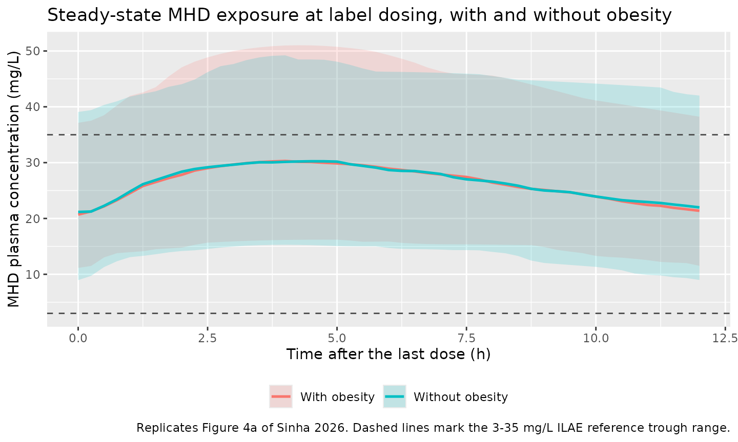
Fig. 4b and Fig. 5: steady-state trough concentrations
ggplot(ss, aes(obesity, ctrough, fill = obesity)) +
  geom_boxplot(alpha = 0.7, outlier.size = 0.6) +
  geom_hline(yintercept = c(3, 35), linetype = "dashed", colour = "grey30") +
  facet_wrap(~ tier, nrow = 1) +
  labs(x = NULL, y = expression(C[trough*","*ss]~of~MHD~(mg/L)), fill = NULL,
       title = "Steady-state MHD trough by dosing tier and obesity status",
       caption = "Replicates Figures 4b and 5 of Sinha 2026.") +
  theme(legend.position = "bottom",
        axis.text.x = element_blank(), axis.ticks.x = element_blank())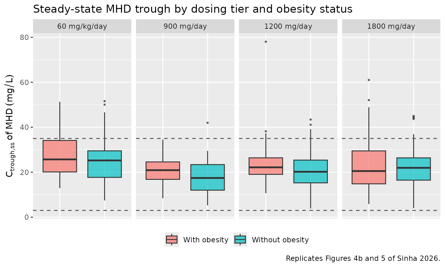
Fig. 7: dosing rate to clearance ratio
Figure 7 plots the individual dosing rate (mg/h) divided by MHD
clearance (L/h) – which, by the steady-state identity derived above,
is the average steady-state MHD concentration (up to the
sf_ft molar factor). The paper’s claim is that this ratio
is comparable across the age and obesity ranges.
The identity gate for this figure is run on a typical-value
(zeroRe) version of the same cohort taken out to 20 doses.
It has to be: at the paper’s six-dose horizon the 80% between-subject
variability on V_MHD leaves a handful of subjects with MHD
half-lives beyond 100 h, who are genuinely not at steady state yet and
for whom the steady-state identity therefore should not hold. Removing
the random effects removes that confound and leaves the structural claim
exposed.
ss_tv <- rxode2::rxSolve(
  rxode2::zeroRe(mod)$simulationModel, build_events(20),
  keep = c("FFM", "WT", "tier", "obesity", "daily_mg"),
  returnType = "data.frame"
) |>
  dplyr::filter(time >= 19 * TAU) |>
  dplyr::group_by(id, daily_mg) |>
  dplyr::summarise(cl_mhd_i = dplyr::first(cl_mhd),
                   cavg = trapz(time, Cc_mhd) / TAU, .groups = "drop") |>
  dplyr::mutate(ratio_analytic = (daily_mg / 24) * SF_FT / cl_mhd_i,
                pct = 100 * (cavg - ratio_analytic) / ratio_analytic)
#> ℹ omega/sigma items treated as zero: 'etalcl', 'etalcl_mhd', 'etalvc_mhd'
#> Warning: multi-subject simulation without without 'omega'

stopifnot(nrow(ss_tv) == nrow(cohort))
stopifnot(max(abs(ss_tv$pct)) < 0.01)
cat(sprintf("Analytic dose-rate/CL ratio reproduces simulated Cavg,ss for all %d subjects; worst deviation %.4f%%.\n",
            nrow(ss_tv), max(abs(ss_tv$pct))))
#> Analytic dose-rate/CL ratio reproduces simulated Cavg,ss for all 400 subjects; worst deviation 0.0005%.
ss <- ss |>
  dplyr::mutate(dose_rate = daily_mg / 24,
                ratio_analytic = dose_rate * SF_FT / cl_mhd_i)

ggplot(ss, aes(WT, ratio_analytic, colour = obesity)) +
  geom_point(alpha = 0.5, size = 1.1) +
  geom_smooth(method = "loess", formula = y ~ x, se = FALSE, linewidth = 0.9) +
  labs(x = "Total body weight (kg)",
       y = expression(Dosing~rate/CL[MHD]==C[avg*","*ss]~(mg/L)),
       colour = NULL,
       title = "Dosing rate to MHD clearance ratio across body size and obesity status",
       caption = "Replicates Figure 7 of Sinha 2026.") +
  theme(legend.position = "bottom")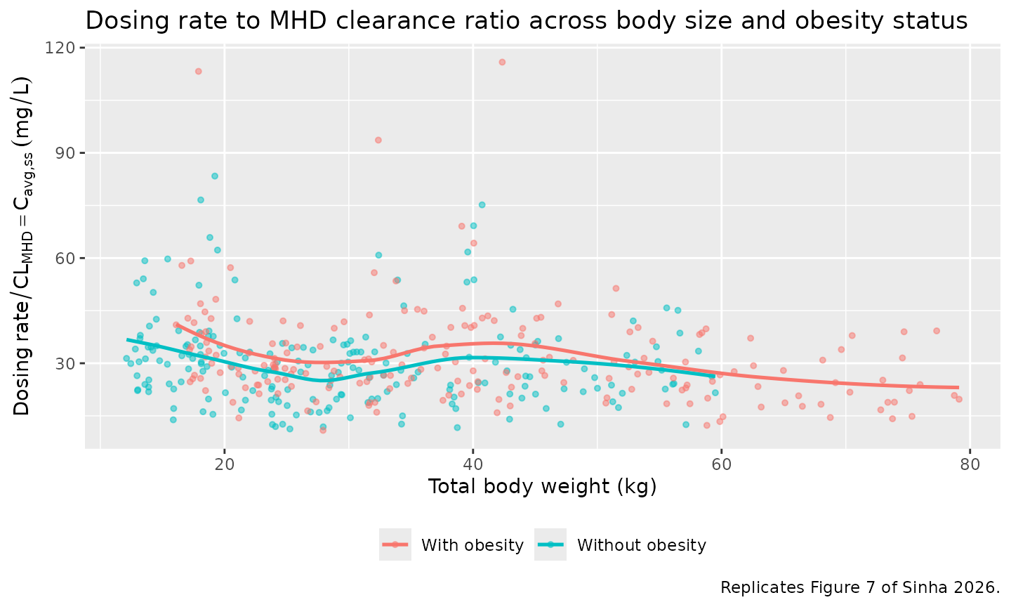
The stopifnot in the preceding chunk is the load-bearing
part: it confirms per subject that the simulated Cavg,ss
equals the analytic dose rate * sf_ft / CL_MHD, which is
what makes Figure 7 a legitimate read-out of average exposure rather
than a proxy for one.
PKNCA validation
A single-dose simulation at the reference body size supplies the standard NCA parameters for both analytes.
ev_sd <- dplyr::bind_rows(
  tibble::tibble(id = 1L, time = 0, amt = 450, evid = 1L, cmt = "depot",
                 dvid = NA_integer_, FFM = 50),
  tibble::tibble(id = 1L, time = seq(0, 168, length.out = 673),
                 amt = NA_real_, evid = 0L, cmt = "central",
                 dvid = 1L, FFM = 50)
) |>
  dplyr::arrange(id, time, dplyr::desc(evid))

sim_sd <- rxode2::rxSolve(
  rxode2::zeroRe(mod)$simulationModel, ev_sd,
  keep = "FFM", returnType = "data.frame"
)
#> ℹ omega/sigma items treated as zero: 'etalcl', 'etalcl_mhd', 'etalvc_mhd'
if (is.null(sim_sd$id)) sim_sd$id <- 1L

dose_df <- data.frame(id = 1L, time = 0, amt = 450)

nca_for <- function(analyte) {
  cdat <- sim_sd |>
    dplyr::select(id, time, conc = dplyr::all_of(analyte)) |>
    dplyr::filter(!is.na(conc))
  res <- PKNCA::pk.nca(PKNCA::PKNCAdata(
    PKNCA::PKNCAconc(cdat, conc ~ time | id, concu = "mg/L", timeu = "hr"),
    PKNCA::PKNCAdose(dose_df, amt ~ time | id, doseu = "mg"),
    intervals = data.frame(start = 0, end = 168, cmax = TRUE, tmax = TRUE,
                           auclast = TRUE, aucinf.obs = TRUE, half.life = TRUE)
  ))
  res$result |> dplyr::mutate(analyte = analyte)
}

nca_all <- dplyr::bind_rows(nca_for("Cc"), nca_for("Cc_mhd"))
stopifnot(nrow(nca_all) > 0)

nca_all |>
  dplyr::filter(PPTESTCD %in% c("cmax", "tmax", "auclast", "aucinf.obs", "half.life")) |>
  dplyr::transmute(
    Analyte = ifelse(analyte == "Cc", "Oxcarbazepine (parent)",
                     "MHD (active metabolite)"),
    `NCA parameter` = PPTESTCD,
    Value = PPORRES
  ) |>
  knitr::kable(
    digits = 3,
    caption = "PKNCA results from a typical-value 450 mg single oral dose at the 50 kg PKWT reference."
)| Analyte | NCA parameter | Value |
|---|---|---|
| Oxcarbazepine (parent) | auclast | 3.479 |
| Oxcarbazepine (parent) | cmax | 0.486 |
| Oxcarbazepine (parent) | tmax | 0.500 |
| Oxcarbazepine (parent) | half.life | 11.385 |
| Oxcarbazepine (parent) | aucinf.obs | 3.479 |
| MHD (active metabolite) | auclast | 148.707 |
| MHD (active metabolite) | cmax | 5.842 |
| MHD (active metabolite) | tmax | 7.250 |
| MHD (active metabolite) | half.life | 11.485 |
| MHD (active metabolite) | aucinf.obs | 148.714 |
Comparison against published exposure values
The paper’s directly comparable published numbers are the interquartile ranges of simulated steady-state MHD trough concentration across the whole 2-20 year virtual population: 13.81-27.13 mg/L with obesity and 13.79-28.16 mg/L without.
iqr_tbl <- ss |>
  dplyr::group_by(obesity) |>
  dplyr::summarise(
    `Simulated Q1` = quantile(ctrough, 0.25),
    `Simulated Q3` = quantile(ctrough, 0.75),
    .groups = "drop"
  ) |>
  dplyr::mutate(
    `Published Q1` = ifelse(obesity == "With obesity", 13.81, 13.79),
    `Published Q3` = ifelse(obesity == "With obesity", 27.13, 28.16)
  ) |>
  dplyr::rename(`Obesity status` = obesity) |>
  dplyr::relocate(`Obesity status`, `Published Q1`, `Simulated Q1`,
                  `Published Q3`, `Simulated Q3`)

knitr::kable(
  iqr_tbl, digits = 2,
  caption = "Interquartile range of steady-state MHD trough concentration at label dosing: this vignette's virtual cohort versus Sinha 2026 Results 3.3."
)| Obesity status | Published Q1 | Simulated Q1 | Published Q3 | Simulated Q3 |
|---|---|---|---|---|
| With obesity | 13.81 | 15.94 | 27.13 | 28.62 |
| Without obesity | 13.79 | 15.51 | 28.16 | 26.96 |
# The paper's headline conclusion is that the two groups' exposures are
# "largely overlapping". Score that on the same quantity and the same
# statistic the paper reports -- the IQR of C_trough,ss -- using the fraction
# of the two IQRs' union that they share. Applying the metric to the paper's
# own published quartiles gives the benchmark to compare against.
iqr_overlap <- function(q1a, q3a, q1b, q3b) {
  inter <- max(0, min(q3a, q3b) - max(q1a, q1b))
  union <- max(q3a, q3b) - min(q1a, q1b)
  inter / union
}
published_overlap <- iqr_overlap(13.81, 27.13, 13.79, 28.16)
simulated_overlap <- iqr_overlap(
  iqr_tbl$`Simulated Q1`[iqr_tbl$`Obesity status` == "With obesity"],
  iqr_tbl$`Simulated Q3`[iqr_tbl$`Obesity status` == "With obesity"],
  iqr_tbl$`Simulated Q1`[iqr_tbl$`Obesity status` == "Without obesity"],
  iqr_tbl$`Simulated Q3`[iqr_tbl$`Obesity status` == "Without obesity"]
)
cat(sprintf("IQR overlap of C_trough,ss between obesity groups: %.0f%% simulated vs %.0f%% published.\n",
            100 * simulated_overlap, 100 * published_overlap))
#> IQR overlap of C_trough,ss between obesity groups: 84% simulated vs 93% published.
stopifnot(published_overlap > 0.9, simulated_overlap > 0.5)

med <- tapply(ss$ctrough, ss$obesity, median)
cat(sprintf("Median C_trough,ss: %.1f mg/L with obesity vs %.1f mg/L without (%.0f%% apart).\n",
            med[["With obesity"]], med[["Without obesity"]],
            100 * abs(diff(med)) / mean(med)))
#> Median C_trough,ss: 21.4 mg/L with obesity vs 22.0 mg/L without (3% apart).

# Every tier should sit inside the ILAE 3-35 mg/L reference trough range.
tier_med <- ss |>
  dplyr::group_by(tier, obesity) |>
  dplyr::summarise(n = dplyr::n(), med = median(ctrough), .groups = "drop")
stopifnot(nrow(tier_med) >= 6, all(tier_med$n > 0),
          all(tier_med$med > 3), all(tier_med$med < 35))
knitr::kable(tier_med |> dplyr::rename(`Dosing tier` = tier,
                                       `Obesity status` = obesity,
                                       `n` = n,
                                       `Median C_trough,ss (mg/L)` = med),
             digits = 2,
caption = "Median steady-state MHD trough per label dose tier; all fall inside the 3-35 mg/L ILAE reference range cited by the paper.")| Dosing tier | Obesity status | n | Median C_trough,ss (mg/L) |
|---|---|---|---|
| 60 mg/kg/day | With obesity | 25 | 25.70 |
| 60 mg/kg/day | Without obesity | 60 | 25.23 |
| 900 mg/day | With obesity | 44 | 20.90 |
| 900 mg/day | Without obesity | 45 | 17.43 |
| 1200 mg/day | With obesity | 38 | 22.17 |
| 1200 mg/day | Without obesity | 42 | 20.20 |
| 1800 mg/day | With obesity | 93 | 20.50 |
| 1800 mg/day | Without obesity | 53 | 21.95 |
Assumptions and deviations
-
Between-subject-variability scale. Sinha 2026
Methods 2.2 defines BSV as “the standard deviation of log-normally
distributed random effects with a zero mean”, and Table 4 reports those
quantities under a column headed “BSV estimates (CV)”. The packaged
ini()therefore treats each reported percentage asomegaitself and squares it (e.g.etalcl ~ 0.51^2), rather than inverting the exact log-normal relationomega^2 = log(CV^2 + 1). Two independent checks support this reading. First, the same table reports the proportional residual errors as “CV%”, and for a NONMEM proportional error the CV is exactlysqrt(sigma^2)with no exponential transform – so the paper’s “CV%” label denotessqrt(variance) * 100. Second, the reported relative standard error on the BSV of CL_MHD is 12%, below thesqrt(2/N) = 14.1%asymptotic RSE expected for a variance estimate at N = 100 subjects. That second check is corroborating rather than decisive – the asymptotic relation is only approximate in the presence of shrinkage – but it points the same way as the Methods definition, which is the primary evidence here. Under the alternative reading the variances would be 12%, 9% and 24% smaller for CL_OXZ, CL_MHD and V_MHD respectively; the structural parameters and all typical-value predictions in this vignette are unaffected either way. -
ESM1 Eq. S4 sign error. The supplement prints the
female paediatric fat-free-mass numerator as
+0.11. It must be-0.11: the multiplier has to converge to 1 at adolescence so Eq. S4 reduces to the adult Eq. S2, and the male numerator is exactly(1 - 0.88) = 0.12. The vignette uses the corrected value and asserts the convergence numerically. This affects only the vignette’s virtual-cohort construction, not any model parameter. -
Molar-mass factors written as exact ratios. The
ESM2 control stream hardcodes the salt factors as 1.00796 and 0.992095.
The model file writes them as
254.28 / 252.27and252.27 / 254.28, matching Methods 2.3.1’s stated derivation. The two forms agree to six significant figures, and the ratio form is exactly reciprocal, which the steady-state identities above require. -
Concentration units. The model works in mg/L
(amounts in mg, volumes in L). The source control stream instead sets
S2 = V2/1000andS3 = V3/1000so that NONMEM predictions come out in ng/mL, matching the 1 ng/mL assay LLOQ. This is a pure scale factor of 1000; mg/L is used here because it is the unit the paper reports every exposure in (trough IQRs, the 3-35 mg/L ILAE range). -
No bioavailability parameter. The source control
stream has no
F1, soFis implicitly 1 – consistent with the Introduction’s statement that OXZ is fully absorbed. Clearances and volumes are therefore absolute, not apparent. -
Parameters with BSV fixed to zero carry no eta.
Table 4 reports BSV of “0 (fixed)” for Ka, Kbt and V_OXZ, matching
0 FIXin the ESM2$OMEGAblock. These are encoded as parameters without an eta rather than as~ fixed(0), which is numerically equivalent and avoids a singular OMEGA. - Virtual cohort is a paper-anchored reconstruction, not the paper’s. The paper sampled 2000 children from the NHANES and Pediatric Trials Network demographic repositories, neither of which was available when this model was built. The cohort here is built from quantities the paper reports: the BMI strata are the Table 2 medians for the mixed-obesity POP01 cohort (18.5 kg/m^2) and the all-obese AED01 cohort (24.6 kg/m^2), and heights follow from a non-obese weight sampled across the span of the label’s weight bands. The weight-to-age mapping – anchors of 12 kg at 3 y, 24.5 kg at 7 y, 34 kg at 11 y, 50 kg at 15 y and 60 kg at 18 y, linearly interpolated – is an assumption of this vignette, not a paper value; the paper sampled uniformly across ten age bins drawn from the two repositories. The trough IQR comparison is therefore a consistency check on the exposure range, not a reproduction of the paper’s Monte-Carlo result, and the simulated IQR overlap between obesity groups is expected to be lower than the paper’s 93% because a deterministic weight-to-age mapping concentrates subjects at the label’s discrete tier boundaries where a real cohort spreads across them. The exact structural identities, the MHD:OXZ exposure ratio and the reference-subject clearances are the checks that do not depend on the cohort construction at all.
-
Residual error in the trough comparison.
Cc_mhdfromrxSolveis an individual prediction without residual error. The published trough IQRs may or may not include the 24% proportional residual; the vignette reports the no-residual values (actrough_ruvcolumn carrying the residual is computed alongside for inspection). -
Steady-state convention. The paper states that “the
simulated exposure post-sixth dose was considered at steady state”, and
the cohort simulation follows that convention so the trough comparison
is scored on the same footing as the published numbers. For a typical
subject the MHD half-life is roughly 10-12 h, so six 12-hourly doses
reach about 99% of true steady state. The 80% between-subject
variability on
V_MHD, however, gives a minority of subjects half-lives beyond 100 h, and those are genuinely still accumulating at six doses – a property of the published model that the paper’s own simulations share. Because of that, the two exact-identity checks are run without random effects (the body-size ladder at 30 doses, the cohort gate at 20), where every subject is fully converged and the structural claim is testable at the 0.01% level. -
Covariates screened but not retained. PNA, PMA (as
a sigmoidal maturation function), serum creatinine, eGFR, phenobarbital,
valproic acid, levetiracetam and topiramate were all tested and none
improved the fit (ESM1 Table S5). They are recorded in the model file’s
covariatesDataExcludedfield rather thancovariateData, since the model does not reference them. The Discussion notes the dataset was underpowered for the enzyme-inducing-antiepileptic effect (n = 6 on phenobarbital, none on carbamazepine) that other oxcarbazepine population PK analyses – includingRodrigues_2017_oxcarbazepinein this package – did detect. -
Race and ethnicity. Race, ethnicity and a
race-white/black indicator were carried in the analysis dataset (ESM2
$INPUT) but no summary is tabulated in the publication, sopopulation$race_ethnicityrecords that they were not reported and the virtual cohort does not stratify on them. -
Erratum – checked and applied. A Correction was
published on 6 January 2026 (Clin Pharmacokinet 2026;65:345, doi:10.1007/s40262-025-01613-1, PMID 41493701). It is a
labelling fix: Eq. 10 of the original was printed as
TV_V,MHD (L) = 50 * (PKWT/50)^0.752– a duplicate of the preceding V_MHD equation – and should readTV_V,OXZ (L) = 33.1 * (PKWT/50)^0.752. No parameter value changes, and the corrected form is exactly what the ESM2 control stream (TVV2 = THETA(2)*(PKWT/50)**THETA(6)withTHETA(2) = 33.1) and Table 4 already specify, so the packaged model was unaffected. The correction is recorded in the model file’sreferencemetadata and independently confirms the V_OXZ / V_MHD assignment and the shared 0.752 volume exponent used here.