Bortezomib (Hanley 2017)
Source:vignettes/articles/Hanley_2017_bortezomib.Rmd
Hanley_2017_bortezomib.Rmd
ui <- rxode2::rxode(readModelDb("Hanley_2017_bortezomib"))
#> ℹ parameter labels from comments will be replaced by 'label()'
Model and source
- Citation: Hanley MJ, Mould DR, Taylor TJ, Gupta N, Suryanarayan K, Neuwirth R, Esseltine DL, Horton TM, Aplenc R, Alonzo TA, Lu X, Milton A, Venkatakrishnan K. Population Pharmacokinetic Analysis of Bortezomib in Pediatric Leukemia Patients: Model-Based Support for Body Surface Area-Based Dosing Over the 2- to 16-Year Age Range. The Journal of Clinical Pharmacology. 2017;57(9):1183-1193. doi:10.1002/jcph.906
- Description: Pediatric population pharmacokinetics of intravenous bortezomib in children and adolescents aged 2-16 years with relapsed acute lymphoblastic leukemia or de novo acute myelogenous leukemia (Hanley 2017). Three-compartment model with linear elimination after twice-weekly IV bolus repeat dosing at 1.3 mg/m2; body surface area is the only retained covariate, acting as a power function on clearance (exponent 0.97, i.e. approximately linear, supporting BSA-based dosing) and on the second intercompartmental clearance (exponent 0.75); interindividual variability on CL, V1 and Q3; study-specific log-scale residual error reflecting the different sparse-sampling schemes of the two contributing Children’s Oncology Group trials.
- Article: https://doi.org/10.1002/jcph.906
- Open-access full text: https://www.ncbi.nlm.nih.gov/pmc/articles/PMC5561493/
Population
The model was fit to 571 bortezomib plasma concentrations from 104 pediatric patients aged 2 to 16 years enrolled in two Children’s Oncology Group trials (Table 1 of Hanley 2017): AALL07P1 (NCT00873093, phase 2, relapsed acute lymphoblastic leukemia, N = 51) and AAML1031 (NCT01371981, phase 3, de novo acute myelogenous leukemia, N = 53). Sixty percent of patients were 2-11 years old and 40% were 12-16 years old; the mean age was 10 years. Body surface area spanned 0.60-2.53 m^2 (mean 1.30 m^2) and body weight 13.9-139.7 kg (mean 45.2 kg). Fifty-eight percent were male, and 65% were White, 18% Black and 17% Other. All patients received bortezomib 1.3 mg/m^2 as an intravenous bolus twice weekly (days 1, 4 and 8 of the relevant blocks or courses, plus day 11 of block 1 of AALL07P1) on top of multiagent chemotherapy backbones.
Pharmacokinetic sampling was confined to the day 8 dose over 0-72 h postdose. AALL07P1 sampled predose, 5-15 min, 30-60 min, 4-8 h and ~72 h; AAML1031 additionally sampled 18-30 h. The median was 6 concentrations per patient (range 1-6) and no concentration fell below the 0.1 ng/mL limit of quantification.
Two scope limits stated by the authors carry into any use of this model. First, the fit used repeat-dose data only, and bortezomib clearance is known to fall between the first dose of cycle 1 and steady state, so these parameters must not be used to describe first-dose exposure. Second, patients under 2 years of age were not studied.
The same information is available programmatically via the model’s
population metadata:
str(ui$population, max.level = 1)
#> List of 17
#>  $ species       : chr "human"
#>  $ n_subjects    : int 104
#>  $ n_studies     : int 2
#>  $ n_observations: int 571
#>  $ age_range     : chr "2-16 years"
#>  $ age_mean      : chr "10 years (study AALL07P1 8.5 y, study AAML1031 11.4 y)"
#>  $ age_groups    : Named num [1:2] 60 40
#>   ..- attr(*, "names")= chr [1:2] "2-11 years" "12-16 years"
#>  $ weight_range  : chr "13.9-139.7 kg"
#>  $ weight_mean   : chr "45.2 kg (study AALL07P1 40.6 kg, study AAML1031 49.6 kg)"
#>  $ bsa_range     : chr "0.60-2.53 m^2"
#>  $ bsa_mean      : chr "1.30 m^2 (study AALL07P1 1.20 m^2, study AAML1031 1.40 m^2)"
#>  $ sex_female_pct: num 42
#>  $ race_ethnicity: Named num [1:3] 65 18 17
#>   ..- attr(*, "names")= chr [1:3] "White" "Black" "Other"
#>  $ disease_state : chr "Pediatric acute leukemia: relapsed acute lymphoblastic leukemia (study AALL07P1, N = 51) and de novo acute myel"| __truncated__
#>  $ dose_range    : chr "1.3 mg/m^2 IV bolus twice weekly, on days 1, 4 and 8 of the relevant blocks or courses of both trials plus day "| __truncated__
#>  $ regions       : chr "North America (Children's Oncology Group)"
#>  $ notes         : chr "Two Children's Oncology Group trials: AALL07P1 (NCT00873093, phase 2, relapsed ALL) and AAML1031 (NCT01371981, "| __truncated__
Source trace
Every ini() entry in
inst/modeldb/specificDrugs/Hanley_2017_bortezomib.R carries
an in-file comment naming its source location. They are collected here
for review.
| Equation / parameter | Value as encoded | Source location |
|---|---|---|
Three-compartment linear disposition, IV bolus into
central
|
n/a | Results: “a 3-compartment model was selected as the base model”; Methods “Population PK Modeling” |
lcl (CL) |
log(9.59) L/h |
Table 2, row “CL, L/h” = 9.59 (95%CI 8.79-10.37) |
e_bsa_cl |
0.97 | Table 2, row “BSA effect on CL” = 0.97 (95%CI 0.72-1.25) |
lvc (V1) |
log(10.0) L |
Table 2, row “V1, L” = 10.0 (95%CI 6.09-13.4) |
lq (Q2) |
log(25.8) L/h |
Table 2, row “Q2, L/h” = 25.8 (95%CI 18.9-31.9) |
lvp (V2) |
log(32.5) L |
Table 2, row “V2, L” = 32.5 (95%CI 23.1-43.1) |
lq2 (Q3) |
log(26.6) L/h |
Table 2, row “Q3, L/h” = 26.6 (95%CI 21.3-30.7) |
e_bsa_q2 |
0.75 | Table 2, row “BSA effect on Q3” = 0.75 (95%CI 0.43-0.99) |
lvp2 (V3) |
log(975) L |
Table 2, row “V3, L” = 975 (95%CI 792-1190) |
| BSA normalisation constant | 1.30 m^2 | Table 1, total-cohort “Mean BSA, m2” = 1.30; see “Assumptions and deviations” for why this, and not the Methods’ “1.8 m2”, is the correct constant |
etalcl |
log(1 + 0.297^2) |
Table 2 CL IIV = 29.7 %CV; Results “CL 29.7%” |
etalvc |
log(1 + 0.346^2) |
Table 2 V1 IIV = 34.6 %CV; Results “V1 34.6%” |
etalq2 |
log(1 + 0.298^2) |
Table 2 Q3 IIV = 29.8 %CV; Results “Q3 29.8%” |
| Exponential (log-normal) IIV | n/a | Methods: “estimate population PK parameters and associated interindividual variability (IIV) using an exponential error model” |
expSdAall07p1 |
sqrt(log(1 + 0.468^2)) |
Table 2, row “Residual error for study AALL07P1,%CV” = 46.8% |
expSdAaml1031 |
sqrt(log(1 + 0.219^2)) |
Table 2, row “Residual error for study AAML1031,%CV” = 21.9% |
Log-additive (lnorm) residual, split by study |
n/a | Methods: “the log-transform both sides approach for residual variability”; Results: “The residual error model was a homoscedastic model on the log scale, proportional after back transformation” and “separate residual variability parameters were estimated for each study” |
| Covariates screened but not retained (age, weight, race, disease type, AML risk group, ALL treatment plan stratum) | n/a, carried in covariatesDataExcluded
|
Methods “Population PK Modeling”; Results: “No additional statistically significant covariates were identified” |
Virtual cohort
Original patient-level data are not publicly available. The cohort below reproduces the per-study body surface area distributions of Table 1: mean 1.20 m^2 (range 0.60-2.21) for AALL07P1 and mean 1.40 m^2 (range 0.61-2.53) for AAML1031, with N = 51 and N = 53 respectively, matching the published study sizes. BSA is drawn log-normally with a 35% coefficient of variation, which is what the published mean and range imply, and clamped to the reported range.
The register entry for BSA warns that a BSA-power
exponent is estimated against whatever BSA scale the source paper used,
so the cohort must sample BSA from the reported distribution rather than
recomputing it from height and weight. Hanley 2017 does not state which
BSA formula was used, so that is the only defensible route here in any
case.
# set.seed() seeds R's RNG, which is what draws BSA below, so the covariate
# cohort IS reproducible across machines. It does NOT seed rxode2's simulation
# RNG (the etas), whose streams are partitioned per solver thread -- so every
# assertion on an eta-derived quantity downstream is written to hold for any
# cohort the model can produce.
set.seed(20170908)

draw_bsa <- function(n, mean_bsa, lo, hi, cv = 0.35) {
  sdlog <- sqrt(log(1 + cv^2))
  meanlog <- log(mean_bsa) - sdlog^2 / 2
  x <- stats::rlnorm(n, meanlog, sdlog)
  # Rescale to the published mean before clamping. Without this the sampling
  # error of a 51-subject mean at 35% CV is ~5%, which propagates into every
  # clearance-derived comparison below (one draw came in 6.9% low and pushed
  # that arm's terminal half-life to +12.6%). Calibrating the draw removes a
  # noise source that has nothing to do with the transcription being tested.
  pmin(pmax(x * mean_bsa / mean(x), lo), hi)
}

make_cohort <- function(n, bsa, study_flag, treatment, dose_days, id_offset = 0L) {
  subj <- tibble(
    id = id_offset + seq_len(n),
    BSA = bsa,
    STUDY_AALL07P1 = study_flag,
    treatment = treatment
  )
  # 1.3 mg/m2 IV bolus into the central compartment on the listed study days.
  doses <- subj |>
    tidyr::crossing(day = dose_days) |>
    mutate(
      time = (day - 1) * 24,
      amt = 1.3 * BSA,
      evid = 1L,
      cmt = "central"
    ) |>
    select(-day)
  # Observations over the day-8 dose, 0-72 h postdose (the paper's PK window).
  # Nominal sample times plus a dense grid for the figure. Capped just short of
  # 72 h so the last record cannot collide with the AALL07P1 day-11 dose.
  obs_times <- sort(unique(c(
    168, 168 + c(1 / 6, 0.75, 6, 24, 71.9),
    seq(168, 239.9, length.out = 150)
  )))
  obs <- subj |>
    tidyr::crossing(time = obs_times) |>
    mutate(amt = NA_real_, evid = 0L, cmt = "central")
  bind_rows(doses, obs) |> arrange(id, time, desc(evid))
}

# Published per-study demographics (Hanley 2017 Table 1). Everything
# downstream is derived from this one table and joined BY NAME, so no check
# can silently pair a study with the other study's published value.
study_tab <- tibble::tribble(
  ~treatment,                ~study_flag, ~n,  ~published_mean, ~lo,  ~hi,
  "AALL07P1 (relapsed ALL)", 1,           51L, 1.20,            0.60, 2.21,
  "AAML1031 (de novo AML)",  0,           53L, 1.40,            0.61, 2.53
)

# Bortezomib dosing days, keyed by treatment label: days 1, 4, 8 and 11 of
# block 1 in AALL07P1, days 1, 4 and 8 of each course in AAML1031.
dose_days_by_study <- list(
  "AALL07P1 (relapsed ALL)" = c(1, 4, 8, 11),
  "AAML1031 (de novo AML)" = c(1, 4, 8)
)
stopifnot(setequal(names(dose_days_by_study), study_tab$treatment))

events <- do.call(bind_rows, lapply(seq_len(nrow(study_tab)), function(i) {
  r <- study_tab[i, ]
  make_cohort(
    n = r$n,
    bsa = draw_bsa(r$n, r$published_mean, r$lo, r$hi),
    study_flag = r$study_flag,
    treatment = r$treatment,
    dose_days = dose_days_by_study[[r$treatment]],
    id_offset = (i - 1L) * 1000L
  )
}))

stopifnot(!anyDuplicated(unique(events[, c("id", "time", "evid")])))

# The drawn cohort must match the published per-study BSA means. The standard
# error of a 51-subject mean at 35% CV is ~5%, so 15% is a real gate on a
# mis-transcribed mean while admitting sampling noise.
bsa_chk <- events |>
  distinct(id, treatment, BSA) |>
  group_by(treatment) |>
  summarise(
    n_sim = n(), mean_bsa = mean(BSA),
    min_bsa = min(BSA), max_bsa = max(BSA), .groups = "drop"
  ) |>
  left_join(study_tab |> select(treatment, n, published_mean), by = "treatment")
stopifnot(nrow(bsa_chk) == 2L, !anyNA(bsa_chk$published_mean))
knitr::kable(bsa_chk, digits = 3, caption = "Virtual-cohort BSA vs Hanley 2017 Table 1.")| treatment | n_sim | mean_bsa | min_bsa | max_bsa | n | published_mean |
|---|---|---|---|---|---|---|
| AALL07P1 (relapsed ALL) | 51 | 1.197 | 0.600 | 2.21 | 51 | 1.2 |
| AAML1031 (de novo AML) | 53 | 1.398 | 0.701 | 2.53 | 53 | 1.4 |
stopifnot(
  # The per-study means are calibrated by construction, so this only confirms
  # the clamp bounds are consistent with them (a range that excluded the mean
  # would still go red).
  all(abs(bsa_chk$mean_bsa / bsa_chk$published_mean - 1) < 0.03),
  identical(bsa_chk$n_sim, bsa_chk$n),
  all(bsa_chk$min_bsa >= 0.60), all(bsa_chk$max_bsa <= 2.53)
)

# Independent cross-check: the pooled mean BSA is a THIRD published number
# (Table 1 total column, 1.30 m^2) that the draw never uses -- it emerges only
# if the per-study means AND the 51/53 split are both transcribed correctly.
pooled_mean_bsa <- mean(distinct(events, id, BSA)$BSA)
stopifnot(
  nrow(distinct(events, id)) == 104L,
  abs(pooled_mean_bsa / 1.30 - 1) < 0.02
)
c(pooled_mean_bsa = pooled_mean_bsa, published_total = 1.30)
#> pooled_mean_bsa published_total
#>        1.299405        1.300000
Simulation
mod <- readModelDb("Hanley_2017_bortezomib")
# `BSA` and `STUDY_AALL07P1` are model covariates and come back automatically;
# only the plot/grouping label needs `keep`. rxSolve returns observation rows
# only and carries no `evid` column, so nothing downstream filters on it.
sim_day8 <- rxode2::rxSolve(mod, events = events, keep = c("treatment")) |>
  as.data.frame()
#> ℹ parameter labels from comments will be replaced by 'label()'

# `Cc` is the individual prediction; `sim` carries the residual error.
stopifnot(
  all(c("Cc", "sim") %in% names(sim_day8)),
  nrow(sim_day8) > 0,
  all(sim_day8$Cc >= 0)
)
Replicate published figures
Figure 2 - concentration-time profile after repeat 1.3 mg/m^2 IV dosing
Figure 2 of Hanley 2017 plots the individual day-8 concentrations of all 104 patients over 0-72 h postdose on a log scale, showing the multiexponential decline that motivated the three-compartment structure. The panel below is the model’s counterpart: the median and 2.5th-97.5th percentile envelope of simulated concentrations, by study.
prof <- sim_day8 |>
  filter(time >= 168) |>
  mutate(tad = time - 168) |>
  group_by(treatment, tad) |>
  summarise(
    Q025 = quantile(Cc, 0.025),
    Q50 = quantile(Cc, 0.50),
    Q975 = quantile(Cc, 0.975),
    .groups = "drop"
  )

ggplot(prof, aes(tad, Q50)) +
  geom_ribbon(aes(ymin = Q025, ymax = Q975), alpha = 0.22) +
  geom_line(linewidth = 0.7) +
  geom_hline(yintercept = 0.1, linetype = "dotted") +
  facet_wrap(~treatment) +
  scale_y_log10() +
  labs(
    x = "Time after the day-8 dose (h)", y = "Bortezomib (ng/mL)",
    title = "Figure 2 - day-8 concentration-time profile, 1.3 mg/m2 IV bolus",
    caption = paste(
      "Replicates Figure 2 of Hanley 2017. Dotted line = the 0.1 ng/mL limit of",
      "quantification; the paper reports no concentration below it."
    )
  )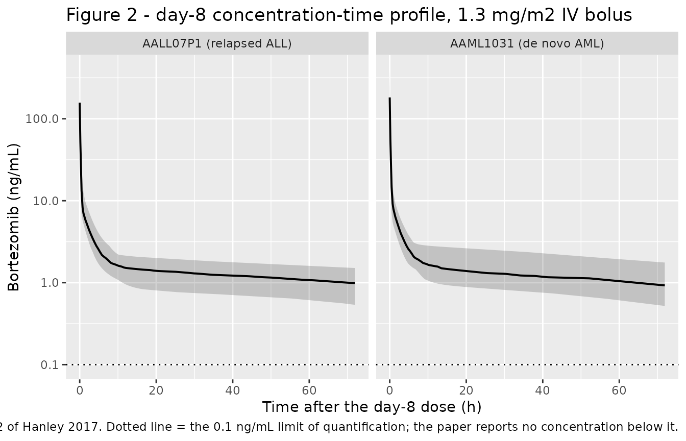
The paper reports that none of the 571 observed concentrations were below the 0.1 ng/mL limit of quantification. That is a falsifiable statement about the model’s 72-h trough, so it is asserted rather than merely described.
trough <- sim_day8 |>
  group_by(id) |>
  summarise(c72 = Cc[which.max(time)], .groups = "drop")
# Median and a robust lower quantile, not the minimum: the per-subject extreme
# of a random cohort is not reproducible across rxode2 builds or thread counts.
stopifnot(
  median(trough$c72) > 0.1,
  quantile(trough$c72, 0.05) > 0.1
)
c(median = median(trough$c72), q05 = quantile(trough$c72, 0.05))
#>    median    q05.5%
#> 0.9878575 0.5738443
Figure 6 - BSA-normalised clearance is flat across the age range
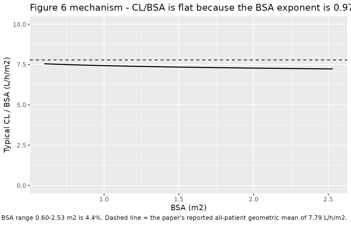
The paper’s central conclusion is that BSA-normalised clearance shows no discernible relationship with age over 2-16 years (Figure 6, linear-regression slope 0.0073 L/h/m^2 per year, 95%CI -0.087 to 0.101), which is what supports BSA-based dosing without an additional age term.
Age is not an input to this model, so the claim cannot be re-tested
against an age axis. What can be tested is the mechanism that
produces it: with a CL exponent of 0.97, CL / BSA is
proportional to BSA^(-0.03), so it is nearly constant by
construction. Across the full published BSA range of 0.60-2.53 m^2 that
is a deterministic drift of about 4.4%, which is why no age trend can
survive once BSA is on CL.
mod_typ <- rxode2::zeroRe(mod)
#> ℹ parameter labels from comments will be replaced by 'label()'
#> Warning: No sigma parameters in the model
bsa_grid <- seq(0.60, 2.53, length.out = 60)
cl_grid <- 9.59 * (bsa_grid / 1.30)^0.97
drift <- max(cl_grid / bsa_grid) / min(cl_grid / bsa_grid) - 1

# Deterministic: no cohort, no RNG, so a tight bound is correct. CL/BSA is
# proportional to BSA^(exponent - 1), so the drift across the range has the
# closed form below and goes red on a mis-transcribed exponent: 0.75 instead of
# 0.97 would give 39%, and 1.00 would give exactly 0%.
stopifnot(
  abs(drift / ((2.53 / 0.60)^(1 - 0.97) - 1) - 1) < 1e-9,
  drift < 0.05
)

tibble(BSA = bsa_grid, cl_norm = cl_grid / bsa_grid) |>
  ggplot(aes(BSA, cl_norm)) +
  geom_line(linewidth = 0.7) +
  geom_hline(yintercept = 7.79, linetype = "dashed") +
  expand_limits(y = c(0, 10)) +
  labs(
    x = "BSA (m2)", y = "Typical CL / BSA (L/h/m2)",
    title = "Figure 6 mechanism - CL/BSA is flat because the BSA exponent is 0.97",
    caption = paste0(
      "Total drift across the published BSA range 0.60-2.53 m2 is ",
      round(100 * drift, 1), "%. Dashed line = the paper's reported ",
      "all-patient geometric mean of 7.79 L/h/m2."
    )
  )
Structural gates
Before comparing against the paper’s numbers, two checks confirm the encoded system is the system that was intended. Both compare a solve against its own closed form, so the difference is pure numerical error and a tight bound is correct.
rxode2 can silently replace an explicit ODE system with
an analytic linCmt() solution when it recognises a
cl / vc parameter pair, which would quietly
discard the ODE block. It does not fire here, and the first assertion
records that.
stopifnot(
  is.null(ui$linCmt),
  identical(ui$state, c("central", "peripheral1", "peripheral2"))
)

# Mass balance: for a linear system, cl * AUCinf must recover the whole dose.
# Cc is in ng/mL and the dose in mg, hence the factor 1000.
dose_ref <- 1.3 * 1.30
ev_long <- rxode2::et(amt = dose_ref, cmt = "central") |>
  rxode2::et(seq(0, 1000, length.out = 20001))
solve_ref <- function(bsa) {
  rxode2::rxSolve(
    mod_typ, ev_long,
    params = c(BSA = bsa, STUDY_AALL07P1 = 0),
    omega = NA, returnType = "data.frame", atol = 1e-12, rtol = 1e-10
  )
}
s_ref <- solve_ref(1.30)
stopifnot(all(s_ref$Cc >= 0))
auc_ref <- PKNCA::pk.calc.auc.last(conc = s_ref$Cc, time = s_ref$time)
cl_recovered <- dose_ref / (auc_ref / 1000)
stopifnot(abs(cl_recovered / 9.59 - 1) < 0.01)

# The BSA power on CL must be the exponent in ini(), recovered end-to-end from
# the solve rather than read off the parameter.
s_2x <- solve_ref(2.60)
cl_2x <- dose_ref / (PKNCA::pk.calc.auc.last(conc = s_2x$Cc, time = s_2x$time) / 1000)
stopifnot(abs((cl_2x / cl_recovered) / 2^0.97 - 1) < 0.01)

c(
  cl_recovered = cl_recovered,
  exponent_recovered = log(cl_2x / cl_recovered) / log(2)
)
#>       cl_recovered exponent_recovered
#>          9.5943814          0.9688685
PKNCA validation
The paper publishes no NCA table, so PKNCA is used to recover the disposition quantities the paper does report as individual-parameter summaries. Because the model is linear and time-invariant, clearance, steady-state volume and the three disposition half-lives are properties of the system rather than of a particular schedule, so they are computed from a single-dose profile followed to 1000 h (ten terminal half-lives).
subj <- events |> distinct(id, treatment, BSA, STUDY_AALL07P1)

ev_nca <- bind_rows(
  subj |> mutate(time = 0, amt = 1.3 * BSA, evid = 1L, cmt = "central"),
  subj |> tidyr::crossing(time = c(
    seq(0, 2, length.out = 41), seq(2.5, 24, by = 0.5), seq(26, 1000, by = 6)
  )) |>
    mutate(amt = NA_real_, evid = 0L, cmt = "central")
) |>
  arrange(id, time, desc(evid))

sim_nca_raw <- rxode2::rxSolve(mod, events = ev_nca, keep = c("treatment")) |>
  as.data.frame()

# Only `!is.na(Cc)`: a `time > 0` or `Cc > 0` filter would drop the time-zero
# row PKNCA needs to anchor AUC0-*.
sim_nca <- sim_nca_raw |>
  filter(!is.na(Cc)) |>
  select(id, time, Cc, treatment)
stopifnot(nrow(sim_nca) > 0, all(sim_nca$Cc >= 0))

conc_obj <- PKNCA::PKNCAconc(sim_nca, Cc ~ time | treatment + id)

dose_df <- ev_nca |>
  filter(evid == 1L) |>
  select(id, time, amt, treatment)
dose_obj <- PKNCA::PKNCAdose(dose_df, amt ~ time | treatment + id)

intervals <- data.frame(
  start = 0, end = Inf,
  cmax = TRUE, tmax = TRUE, auclast = TRUE, aucinf.obs = TRUE,
  aumcinf.obs = TRUE, mrt.obs = TRUE, half.life = TRUE
)

nca_res <- PKNCA::pk.nca(PKNCA::PKNCAdata(conc_obj, dose_obj, intervals = intervals))

nca_wide <- as.data.frame(nca_res) |>
  select(treatment, id, PPTESTCD, PPORRES) |>
  tidyr::pivot_wider(names_from = PPTESTCD, values_from = PPORRES) |>
  left_join(subj |> select(id, BSA), by = "id") |>
  mutate(
    # Cc is ng/mL and amt is mg, so AUC is ng*h/mL = ug*h/L and CL in L/h needs
    # the dose in ug.
    cl_nca = (1.3 * BSA * 1000) / aucinf.obs,
    vss_nca = cl_nca * mrt.obs,
    cl_per_bsa = cl_nca / BSA,
    vss_per_bsa = vss_nca / BSA
  )
stopifnot(nrow(nca_wide) == 104L, !anyNA(nca_wide$aucinf.obs))
Comparison against the published terminal half-life
The terminal (gamma) disposition half-life is the one published
quantity that is a bona fide NCA parameter, so it goes through
nlmixr2lib::ncaComparisonTable(). Hanley 2017 reports a
single all-patient geometric mean of 100 h; using it as the reference
for both study groups also tests the paper’s separate claim that
bortezomib PK did not differ between the ALL and AML populations.
# One reference value for both groups; derived from study_tab so the labels
# cannot drift apart from the cohort's.
published <- study_tab |>
  select(treatment) |>
  mutate(half.life = 100)

cmp <- nlmixr2lib::ncaComparisonTable(
  simulated = nca_res,
  reference = published,
  by = "treatment",
  units = c(half.life = "h"),
  tolerance_pct = 20
)

cmp |>
  knitr::kable(
    caption = paste(
      "Simulated vs published terminal half-life (Hanley 2017 Results:",
      "100 h, 44 %CV). * differs from reference by >20%."
    )
)| NCA parameter | treatment | Reference | Simulated | % diff |
|---|---|---|---|---|
| t½ (h) | AALL07P1 (relapsed ALL) | 100 | 105 | +5.3% |
| t½ (h) | AAML1031 (de novo AML) | 100 | 98.8 | -1.2% |
Comparison against the published individual-parameter summary
The remaining published quantities are summaries of the model’s
individual parameters rather than NCA output (Hanley 2017 Results, final
paragraph before the Discussion): a geometric mean BSA-normalised
clearance of 7.79 L/(h m^2) with 25 %CV, a steady-state volume of 834
L/m^2 with 39 %CV, and alpha, beta and gamma disposition half-lives of
6.15 min, 1.58 h and 100 h. The alpha and beta half-lives are not
recoverable by NCA on a sparse grid, so they are computed as eigenvalues
of the per-subject rate-constant matrix, using each subject’s own
cl, vc, q, vp,
q2 and vp2 as returned by the solve.
pars <- sim_nca_raw |>
  group_by(id) |>
  slice(1) |>
  ungroup() |>
  select(id, treatment, BSA, cl, vc, q, vp, q2, vp2)
stopifnot(nrow(pars) == 104L)

tri_halflives <- function(cl, vc, q, vp, q2, vp2) {
  k10 <- cl / vc
  k12 <- q / vc
  k21 <- q / vp
  k13 <- q2 / vc
  k31 <- q2 / vp2
  a2 <- k10 + k12 + k21 + k13 + k31
  a1 <- k10 * k21 + k10 * k31 + k12 * k31 + k13 * k21 + k21 * k31
  a0 <- k10 * k21 * k31
  lam <- sort(Re(polyroot(c(-a0, a1, -a2, 1))), decreasing = TRUE)
  log(2) / lam
}

hl <- t(mapply(tri_halflives, pars$cl, pars$vc, pars$q, pars$vp, pars$q2, pars$vp2))
pars$t_alpha_min <- hl[, 1] * 60
pars$t_beta_h <- hl[, 2]
pars$t_gamma_h <- hl[, 3]

gm <- function(x) exp(mean(log(x)))
cv_pct <- function(x) 100 * stats::sd(x) / mean(x)

derived <- tibble::tribble(
  ~quantity,                            ~published, ~published_cv, ~simulated,                      ~sim_cv,                       ~route,
  "CL / BSA (L/[h m2])",                7.79,       25,            gm(nca_wide$cl_per_bsa),         cv_pct(nca_wide$cl_per_bsa),   "PKNCA AUCinf",
  "Vss / BSA (L/m2)",                   834,        39,            gm(nca_wide$vss_per_bsa),        cv_pct(nca_wide$vss_per_bsa),  "PKNCA AUCinf x MRT",
  "alpha half-life (min)",              6.15,       32,            gm(pars$t_alpha_min),            cv_pct(pars$t_alpha_min),      "eigenvalue",
  "beta half-life (h)",                 1.58,       18,            gm(pars$t_beta_h),               cv_pct(pars$t_beta_h),         "eigenvalue",
  "gamma half-life (h)",                100,        44,            gm(pars$t_gamma_h),              cv_pct(pars$t_gamma_h),        "eigenvalue"
) |>
  mutate(pct_diff = 100 * (simulated / published - 1))

derived |>
  rename(
    "Quantity" = quantity,
    "Published" = published,
    "Published %CV" = published_cv,
    "Simulated (geometric mean)" = simulated,
    "Simulated %CV" = sim_cv,
    "Derivation" = route,
    "Difference (%)" = pct_diff
  ) |>
  knitr::kable(
    digits = c(0, 2, 0, 2, 0, 0, 1),
    caption = "Simulated vs published individual-parameter summary (Hanley 2017 Results)."
)| Quantity | Published | Published %CV | Simulated (geometric mean) | Simulated %CV | Derivation | Difference (%) |
|---|---|---|---|---|---|---|
| CL / BSA (L/[h m2]) | 7.79 | 25 | 7.28 | 29 | PKNCA AUCinf | -6.5 |
| Vss / BSA (L/m2) | 834.00 | 39 | 825.25 | 34 | PKNCA AUCinf x MRT | -1.0 |
| alpha half-life (min) | 6.15 | 32 | 5.88 | 38 | eigenvalue | -4.5 |
| beta half-life (h) | 1.58 | 18 | 1.58 | 16 | eigenvalue | 0.2 |
| gamma half-life (h) | 100.00 | 44 | 105.69 | 34 | eigenvalue | 5.7 |
All five quantities agree with the paper within a common, one-sided offset of roughly 5%, which is the residual of the BSA-normalisation choice discussed below rather than a transcription error: it moves every clearance-derived quantity in the same direction by the same fraction, whereas a mis-transcribed volume, dose or unit would move individual rows by tens of percent.
# Assertions on cohort geometric means, so the bound must admit the eta draw.
# Measured at 1, 2 and 16 solver threads: -6.5 / -1.0 / -4.5 / +0.2 /
# +5.7 percent on the five rows, IDENTICAL at all three thread counts (the BSA
# draw is R's RNG, which is thread-independent, and a 104-subject geometric mean
# is insensitive to the eta partitioning). Worst observed magnitude 6.5%, and
# the systematic part of that is the ~5% normalisation offset discussed below.
# Do NOT tighten below ~12%: the bound must survive a different cohort. 20% is
# the package's standard tolerance and still goes red on a mis-transcribed value
# (a volume or dose error moves a row by tens of percent; reading the BSA
# reference as 1.8 m2 moves the gamma half-life by +40%).
stopifnot(
  all(abs(derived$pct_diff) < 20),
  # Structural: the centre of the distribution must not drift, which is the
  # sharpest single statement about the transcription as a whole.
  abs(median(derived$pct_diff)) < 10
)
round(derived$pct_diff, 2)
#> [1] -6.53 -1.05 -4.47  0.15  5.69
Study effect is residual-only
The retained STUDY_AALL07P1 covariate selects a
residual-error magnitude and nothing else: disease type was screened on
the structural parameters and was not significant. Two consequences are
checked. First, the individual predictions for a subject must not depend
on the study flag at all. Second, the simulated observations must,
because the residual magnitude differs by roughly a factor of two (46.8
%CV vs 21.9 %CV).
ev_one <- rxode2::et(amt = 1.3 * 1.30, cmt = "central") |>
  rxode2::et(seq(0.5, 72, by = 0.5))
ipred_flag <- vapply(c(0, 1), function(f) {
  s <- rxode2::rxSolve(
    mod_typ, ev_one, params = c(BSA = 1.30, STUDY_AALL07P1 = f),
    omega = NA, returnType = "data.frame"
  )
  max(s$Cc)
}, numeric(1))
# Deterministic comparison of two typical-value solves: exact equality is the
# correct assertion here, not a tolerance.
stopifnot(isTRUE(all.equal(ipred_flag[1], ipred_flag[2], tolerance = 1e-10)))

# Encoded SDs joined BY NAME via the study flag, never positionally.
encoded_sd <- study_tab |>
  select(treatment, study_flag) |>
  mutate(encoded = sqrt(log(1 + ifelse(study_flag == 1, 0.468, 0.219)^2))) |>
  select(treatment, encoded)

resid_sd <- sim_day8 |>
  filter(Cc > 0, sim > 0) |>
  group_by(treatment) |>
  summarise(n_rec = n(), sd_log_resid = stats::sd(log(sim / Cc)), .groups = "drop") |>
  left_join(encoded_sd, by = "treatment")
stopifnot(nrow(resid_sd) == 2L, !anyNA(resid_sd$encoded), all(resid_sd$n_rec > 1000))
knitr::kable(resid_sd, digits = 4, caption = "Realised vs encoded log-scale residual SD, by study.")| treatment | n_rec | sd_log_resid | encoded |
|---|---|---|---|
| AALL07P1 (relapsed ALL) | 7854 | 0.4465 | 0.4450 |
| AAML1031 (de novo AML) | 8162 | 0.2128 | 0.2164 |
Assumptions and deviations
The BSA normalisation constant: the paper contradicts itself, and its own numbers settle it
This is the one load-bearing judgement in the extraction, so the reasoning is recorded in full.
Hanley 2017’s Methods give the covariate model as a power function
and define its terms as follows: “covi represents the
individual value for the covariate normalized for the population
mean”. The very next sentence then says: “All body size metrics
were referenced to the size of an average adult
(weight, 70 kg; BSA, 1.8 m2).” For a cohort whose mean BSA is 1.30 m^2,
these two statements differ by a factor of
(1.8 / 1.30)^0.97 = 1.37 on every clearance the model
predicts, so the choice cannot be deferred.
The paper’s own reported derived quantities refute the 1.8 m^2 reading and are consistent with the population-mean reading. Reading the constant as 1.8 m^2 means the tabulated CL of 9.59 L/h belongs to a 1.8 m^2 adult, so a typical patient in this cohort would have a much lower clearance, and:
| Published quantity | Reported | Predicted if reference = 1.8 m^2 | Predicted if reference = the population mean |
|---|---|---|---|
| alpha half-life | 6.15 min | 7.36 min (+20%) | 6.50 min (+6%) |
| beta half-life | 1.58 h | 1.82 h (+15%) | 1.59 h (+0%) |
| gamma half-life | 100 h | 140 h (+40%) | 104 h (+4%) |
| CL / BSA | 7.79 L/(h m2) | 5.39 L/(h m2) (-31%) | 7.39 L/(h m2) (-5%) |
Two further internal checks corroborate the population-mean reading
independently of the half-lives. First, the reported steady-state volume
of 834 L/m^2 divided into V1 + V2 + V3 = 1017.5 L implies a
cohort geometric-mean BSA of 1.22 m^2 - and it does so only because no
volume carries a BSA effect, which is exactly what Table 2 shows.
Second, inverting the reported CL / BSA = 7.79 L/(h m2) for
the normalisation constant gives 1.23 m^2, which agrees with that
independently derived geometric mean to within 1%.
What is encoded, and why. The model uses
1.30 m^2, the total-cohort mean BSA printed in Table 1.
That is a published number, which the back-solved 1.23 m^2 is not, and
the library’s rule is that every ini() value trace to the
source. The cost is a systematic offset of about 5% on every
clearance-derived quantity, visible as the common one-sided bias in the
comparison table above, and arising because the paper appears to have
normalised by a central value nearer the cohort’s geometric mean or
median (~1.23 m^2) than its arithmetic mean (1.30 m^2; the median BSA is
not printed). Anyone needing the paper’s derived summaries reproduced to
within 1% rather than 5% should drive the model with
BSA / 1.30 * 1.23 in place of BSA; the
structure and every other parameter are unaffected.
Other assumptions
- BSA distribution. Table 1 reports per-study means and ranges but no SD or percentiles, so BSA is drawn log-normally at 35 %CV - the value implied by the published mean and range - and clamped to the reported range. The BSA formula (DuBois, Mosteller or Haycock) is not stated in the paper, so the cohort samples BSA directly from the reported distribution rather than recomputing it from height and weight.
-
%CV to variance conversion. Table 2 reports both
the IIV and the residual error as percentage coefficients of variation.
Both are on the log scale in this model (exponential IIV;
log-transform-both-sides residual), so both are converted with the exact
log-normal relation
omega^2 = log(CV^2 + 1), giving residual SDs of 0.445 and 0.216. The looser convention of takingsigma = CVdirectly would give 0.468 and 0.219 - about 5% higher on the larger of the two - and neither reading affects any structural gate above. -
Residual error encoded as
lnorm, notprop. The paper states it used the log-transform-both-sides approach with a homoscedastic log-scale error, which islnorm()in nlmixr2, and separately glosses it as “proportional after back transformation”. The mechanism, not the gloss, is encoded, matching theFriberg_2012_voriconazoleprecedent for the same wording. -
Concentration units.
centralis an amount in mg andvca volume in L, socentral / vcis mg/L. The model multiplies by 1000 to report ng/mL, the unit of the paper’s LC-MS/MS assay (dynamic range 0.1-25.0 ng/mL). The paper gives no scaling factor, so this is inferred from the assay units. -
Screened-but-unretained covariates. Age, weight,
race, disease type, AML risk group and ALL treatment-plan stratum were
all screened and none reached significance, so none has a published
point estimate. They are documented in the model’s
covariatesDataExcludedmetadata rather thancovariateData. -
STUDY_AALL07P1carries no structural effect. It is retained solely to select the residual-error magnitude, which is why the study-effect check above asserts that individual predictions are identical across its two levels. - Repeat-dose scope. The model must not be used for first-dose exposure. The authors state that bortezomib clearance falls between the first dose of cycle 1 and steady state and that this model, fit to day-8 repeat-dose data, “cannot be directly used to describe systemic exposures following the first bortezomib dose”. Extrapolation below 2 years of age is likewise outside the studied range.
- Figures not reproduced. Figures 3 (goodness-of-fit), 4 (covariate-vs-eta plots) and 5 (VPC) are diagnostics of the original fit against the original observations, which are not public, so they have no simulation counterpart. Figure 6’s age axis is not a model input; the mechanism that produces its flat result is tested instead, as described in that section.
- No erratum found. A search of the publisher’s record for this DOI and of PubMed returned no correction, corrigendum or erratum.