Glenzocimab (Renaud 2020)
Source:vignettes/articles/Renaud_2020_glenzocimab.Rmd
Renaud_2020_glenzocimab.RmdModel and source
- Citation: Renaud L, Lebozec K, Voors-Pette C, Dogterom P, Billiald P, Jandrot Perrus M, Pletan Y, Machacek M. Population Pharmacokinetic/Pharmacodynamic Modeling of Glenzocimab (ACT017) a Glycoprotein VI Inhibitor of Collagen-Induced Platelet Aggregation. J Clin Pharmacol. 2020;60(9):1198-1208. doi:10.1002/jcph.1616
- Description: Two-compartment population PK model with a direct (immediate) Imax model of ex vivo collagen-induced platelet aggregation for glenzocimab (ACT017), an anti-GPVI Fab, in healthy volunteers (Renaud 2020)
- Article: https://doi.org/10.1002/jcph.1616 (open access, PMC7496554)
Glenzocimab (ACT017) is a humanized Fab directed against platelet glycoprotein VI (GPVI). Renaud 2020 fit a joint population PK/PD model in Monolix 2018R1 to plasma glenzocimab concentrations and ex vivo collagen-induced platelet aggregation (light-transmission aggregometry, % aggregation) from the phase I single-ascending-dose study.
Population
36 healthy volunteers received glenzocimab (6 per dose group at 62.5, 125, 250, 500, 1000 and 2000 mg; 12 further placebo subjects did not contribute to the model). 36.1% were female, 91.7% White; median age 56 years (22-63), median body weight 74 kg (52-107), median creatinine 0.77 mg/dL (0.46-1.2), median platelet count 207 x 10^9/L (159-323); 19% had mild renal impairment by eGFR (Renaud 2020 Table 1). Every dose was a 6-hour IV infusion with 25% of the dose in the first 15 minutes and 75% over the remaining 5 h 45 min. 390 PK and 404 PD observations were analysed.
The same information is available programmatically via
readModelDb("Renaud_2020_glenzocimab")()$population.
Source trace
| Equation / parameter | Value | Source location |
|---|---|---|
| Two-compartment linear PK, central elimination | – | Methods, ‘Population PK and PD Base Structural Model’ |
| Two-rate infusion (25% over 15 min, 75% over 5.75 h) | – | Methods, same section |
PPA = Base_PPA - Imax * C / (IC50 + C) |
– | Eq. 1 |
Power covariate model
phi_pop * (cov/ref)^beta * exp(eta)
|
– | Eq. 3 and Table 2 footnotes c-j |
Combined error
yobs = ypred + (a1 + b1 * ypred) * eps
|
– | Eq. 5 |
| Logit-normal PD error on 0-100% | – | Eq. 6 |
lcl |
log(2.67) L/h | Table 2 |
lvc |
log(4.1) L | Table 2 |
lq |
log(0.626) L/h | Table 2 |
lvp |
log(6.89) L | Table 2 |
lrbase (Base_PPA) |
log(79.8) % | Table 2 |
lic50 |
log(0.924) ug/mL | Table 2 |
limax |
log(72.9) % | Table 2 |
e_age_cl, e_wt_cl,
e_creat_cl
|
-0.304, 1.09, -0.566 | Table 2 (footnotes c, d, e) |
e_wt_vc |
0.694 | Table 2 (footnote f) |
e_age_q, e_wt_q
|
-0.318, 0.812 | Table 2 (footnotes g, h) |
e_dose_ic50 |
-0.989 | Table 2 (footnote i, reference 500 mg) |
e_plt_imax |
0.17 | Table 2 (footnote j, reference 220 x 10^9/L) |
| omega CL, V1, Q, V2, IC50 (SD) | 0.182, 0.148, 0.144, 0.265, 1.35 | Table 2 |
| r V1-CL, Q-CL, V1-Q | 0.626, 0.796, 0.84 | Table 2 |
addSd, propSd
|
0.0869 ug/mL, 0.0514 | Table 2 (a1, b1) |
addSd_PPA |
0.778 (logit scale) | Table 2 (a2) |
| Covariate references 70 kg, 50 y, 0.79 mg/dL, 220 x 10^9/L | – | Methods, ‘Population PK/PD Stochastic Model’ |
Deterministic checks against the paper’s derived values
The paper derives an initial half-life of 0.84 h and a terminal half-life of 9.6 h from the typical parameters, an IC50 of 0.47 ug/mL for a 1000 mg dose, and an Imax that varies from 69% to 78% over the observed platelet-count range (159-323 x 10^9/L). All four follow in closed form from the packaged parameters.
mod <- rxode2::rxode(readModelDb("Renaud_2020_glenzocimab"))
#> ℹ parameter labels from comments will be replaced by 'label()'
p <- mod$theta
cl <- exp(p[["lcl"]])
vc <- exp(p[["lvc"]])
q <- exp(p[["lq"]])
vp <- exp(p[["lvp"]])
k10 <- cl / vc
k12 <- q / vc
k21 <- q / vp
s <- k10 + k12 + k21
lambda <- (s + c(1, -1) * sqrt(s^2 - 4 * k10 * k21)) / 2
thalf <- log(2) / lambda
ic50_1000 <- exp(p[["lic50"]]) * (1000 / 500)^p[["e_dose_ic50"]]
imax_range <- exp(p[["limax"]]) * (c(159, 323) / 220)^p[["e_plt_imax"]]

knitr::kable(
  data.frame(
    Quantity = c(
      "Initial half-life (h)", "Terminal half-life (h)",
      "IC50 at 1000 mg (ug/mL)", "Imax at PLT 159 (%)", "Imax at PLT 323 (%)"
    ),
    Packaged = signif(c(thalf, ic50_1000, imax_range), 3),
    Paper = c(0.84, 9.6, 0.47, 69, 78)
  )
)| Quantity | Packaged | Paper |
|---|---|---|
| Initial half-life (h) | 0.842 | 0.84 |
| Terminal half-life (h) | 9.640 | 9.60 |
| IC50 at 1000 mg (ug/mL) | 0.466 | 0.47 |
| Imax at PLT 159 (%) | 69.000 | 69.00 |
| Imax at PLT 323 (%) | 77.800 | 78.00 |
Dosing helper
The phase I regimen is two consecutive zero-order infusions into
central. Observation rows carry dvid = 1: the
model has two error endpoints (Cc and PPA),
and with dvid = 1 on every observation row the solve
returns both as columns. The DOSE covariate is the
subject’s total dose (mg).
make_events <- function(ids, dose, obs_times, inf_h = 6, first_frac = 0.25) {
  one <- function(i) {
    doses <- data.frame(
      id = i, time = c(0, 0.25),
      amt = dose * c(first_frac, 1 - first_frac),
      rate = dose * c(first_frac / 0.25, (1 - first_frac) / (inf_h - 0.25)),
      evid = 1L, cmt = "central", dvid = NA_integer_
    )
    obs <- data.frame(
      id = i, time = obs_times, amt = 0, rate = 0,
      evid = 0L, cmt = NA_character_, dvid = 1L
    )
    dplyr::bind_rows(doses, obs)
  }
  ev <- dplyr::bind_rows(lapply(ids, one))
  ev$DOSE <- dose
  ev
}

# Truncated-normal covariate draw (reject and redraw), centred on the Table 1
# medians with SD = range / 4; the paper sampled from the phase I means and SDs
# truncated at the observed extremes but printed only medians and ranges.
draw_trunc <- function(n, centre, lo, hi) {
  x <- rnorm(n, centre, (hi - lo) / 4)
  bad <- x < lo | x > hi
  while (any(bad)) {
    x[bad] <- rnorm(sum(bad), centre, (hi - lo) / 4)
    bad <- x < lo | x > hi
  }
  x
}

make_cohort <- function(ids) {
  n <- length(ids)
  data.frame(
    id = ids,
    WT = draw_trunc(n, 74, 52, 107),
    AGE = draw_trunc(n, 56, 22, 63),
    CREAT = draw_trunc(n, 0.77, 0.46, 1.2),
    PLT = draw_trunc(n, 207, 159, 323)
  )
}
Virtual phase I cohort and VPC-style profiles
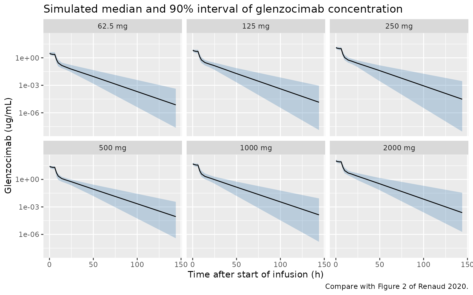
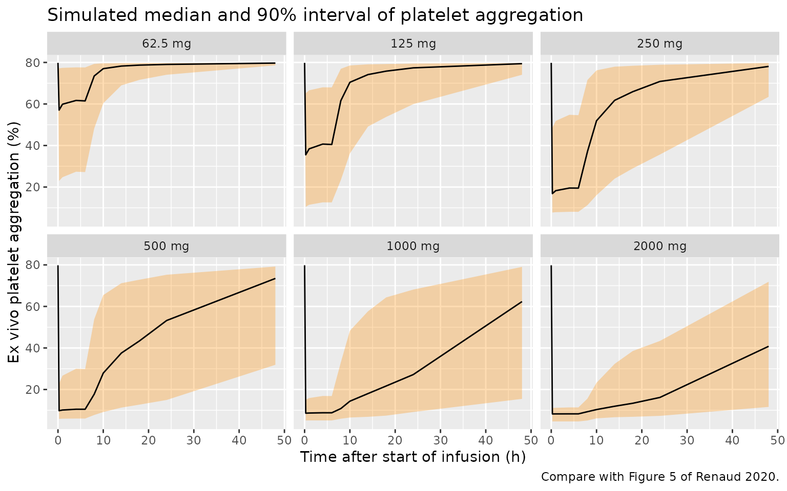
100 virtual subjects per phase I dose group, sampled at the phase I PK/PD schedule (pre-dose, 0.25, 1, 4, 6, 8, 10, 14, 18, 24, 48 and 144 h).
set.seed(20200901) # covariate draws (base R)
rxode2::rxSetSeed(20200901) # etas
doses_p1 <- c(62.5, 125, 250, 500, 1000, 2000)
n_arm <- 100
obs_p1 <- c(0, 0.25, 1, 4, 6, 8, 10, 14, 18, 24, 48, 144)

ev_p1 <- dplyr::bind_rows(lapply(seq_along(doses_p1), function(k) {
  ids <- (k - 1) * n_arm + seq_len(n_arm)
  make_events(ids, doses_p1[k], obs_p1)
}))
cov_p1 <- make_cohort(unique(ev_p1$id))
ev_p1 <- dplyr::left_join(ev_p1, cov_p1, by = "id")

# Tight tolerances: at 144 h a fast-clearing subject is ~15 half-lives out, and
# default-tolerance ODE noise can turn a ~1e-6 ug/mL value slightly negative.
sim_p1 <- rxode2::rxSolve(mod, ev_p1, returnType = "data.frame", atol = 1e-12, rtol = 1e-10) |>
  dplyr::mutate(id = as.integer(as.character(id))) |>
  dplyr::mutate(dose_group = factor(paste(DOSE, "mg"), levels = paste(doses_p1, "mg")))
The concentration and aggregation profiles are summarised from the
individual predictions Cc and PPA (no residual
error).
prof <- sim_p1 |>
  dplyr::select(dose_group, id, time, Cc, PPA) |>
  tidyr::pivot_longer(c(Cc, PPA), names_to = "endpoint") |>
  dplyr::group_by(dose_group, endpoint, time) |>
  dplyr::summarise(
    q05 = quantile(value, 0.05), q50 = median(value), q95 = quantile(value, 0.95),
    .groups = "drop"
  )

ggplot(dplyr::filter(prof, endpoint == "Cc", time > 0), aes(time, q50)) +
  geom_ribbon(aes(ymin = q05, ymax = q95), alpha = 0.3, fill = "steelblue") +
  geom_line() +
  scale_y_log10() +
  facet_wrap(~dose_group) +
  labs(
    x = "Time after start of infusion (h)", y = "Glenzocimab (ug/mL)",
    title = "Simulated median and 90% interval of glenzocimab concentration",
    caption = "Compare with Figure 2 of Renaud 2020."
  )
ggplot(dplyr::filter(prof, endpoint == "PPA", time <= 48), aes(time, q50)) +
  geom_ribbon(aes(ymin = q05, ymax = q95), alpha = 0.3, fill = "darkorange") +
  geom_line() +
  facet_wrap(~dose_group) +
  labs(
    x = "Time after start of infusion (h)", y = "Ex vivo platelet aggregation (%)",
    title = "Simulated median and 90% interval of platelet aggregation",
    caption = "Compare with Figure 5 of Renaud 2020."
  )
PKNCA validation
Renaud 2020 does not print an NCA table. The checks are therefore (i) that the simulated terminal half-life of a reference subject (70 kg, 50 years, creatinine 0.79 mg/dL) reproduces the paper’s 9.6 h and its AUC(0-inf) reproduces Dose / CL = Dose / 2.67 L/h, and (ii) that exposure in the virtual phase I cohort is dose proportional, as the paper reports (Figure S1).
obs_dense <- sort(unique(c(0, 0.25, seq(0.5, 12, by = 0.5), seq(13, 48, by = 1), seq(52, 144, by = 4))))
ev_typ <- dplyr::bind_rows(lapply(seq_along(doses_p1), function(k) {
  make_events(k, doses_p1[k], obs_dense)
})) |>
  dplyr::mutate(WT = 70, AGE = 50, CREAT = 0.79, PLT = 220)

sim_typ <- rxode2::rxSolve(rxode2::zeroRe(mod), ev_typ, returnType = "data.frame") |>
  dplyr::mutate(id = as.integer(as.character(id))) |>
  dplyr::mutate(treatment = paste(DOSE, "mg"))
#> ℹ omega/sigma items treated as zero: 'etalcl', 'etalvc', 'etalq', 'etalvp', 'etalic50'
#> Warning: multi-subject simulation without without 'omega'

conc_typ <- sim_typ |>
  dplyr::filter(!is.na(Cc)) |>
  dplyr::select(id, time, Cc, treatment)
dose_typ <- ev_typ |>
  dplyr::filter(evid == 1, time == 0) |>
  dplyr::transmute(id, time, dose = DOSE, treatment = paste(DOSE, "mg"))

conc_obj <- PKNCA::PKNCAconc(conc_typ, Cc ~ time | treatment + id, concu = "ug/mL", timeu = "h")
dose_obj <- PKNCA::PKNCAdose(dose_typ, dose ~ time | treatment + id, doseu = "mg")
intervals <- data.frame(
  start = 0, end = Inf, cmax = TRUE, tmax = TRUE,
  aucinf.obs = TRUE, half.life = TRUE
)
nca_typ <- PKNCA::pk.nca(PKNCA::PKNCAdata(conc_obj, dose_obj, intervals = intervals))

sim_nca <- as.data.frame(nca_typ$result) |>
  dplyr::filter(PPTESTCD %in% c("aucinf.obs", "half.life")) |>
  dplyr::select(id, treatment, PPTESTCD, PPORRES)

reference <- data.frame(
  treatment = paste(doses_p1, "mg"),
  aucinf.obs = doses_p1 / 2.67,
  half.life = 9.6
)

cmp <- nlmixr2lib::ncaComparisonTable(
  simulated = sim_nca,
  reference = reference,
  by = "treatment",
  units = c(aucinf.obs = "h*ug/mL", half.life = "h"),
  tolerance_pct = 20
)
knitr::kable(cmp, caption = "Reference subject: simulated NCA vs the paper's typical CL (Dose / 2.67) and terminal half-life (9.6 h).")| NCA parameter | treatment | Reference | Simulated | % diff |
|---|---|---|---|---|
| AUC0-∞ (obs) (h*ug/mL) | 62.5 mg | 23.4 | 23.4 | +0.0% |
| AUC0-∞ (obs) (h*ug/mL) | 125 mg | 46.8 | 46.8 | +0.0% |
| AUC0-∞ (obs) (h*ug/mL) | 250 mg | 93.6 | 93.7 | +0.0% |
| AUC0-∞ (obs) (h*ug/mL) | 500 mg | 187 | 187 | +0.0% |
| AUC0-∞ (obs) (h*ug/mL) | 1000 mg | 375 | 375 | +0.0% |
| AUC0-∞ (obs) (h*ug/mL) | 2000 mg | 749 | 749 | +0.0% |
| t½ (h) | 62.5 mg | 9.6 | 9.61 | +0.1% |
| t½ (h) | 125 mg | 9.6 | 9.61 | +0.1% |
| t½ (h) | 250 mg | 9.6 | 9.61 | +0.1% |
| t½ (h) | 500 mg | 9.6 | 9.61 | +0.1% |
| t½ (h) | 1000 mg | 9.6 | 9.61 | +0.1% |
| t½ (h) | 2000 mg | 9.6 | 9.61 | +0.1% |
chk <- sim_nca |>
  dplyr::left_join(
    tidyr::pivot_longer(reference, -treatment, names_to = "PPTESTCD", values_to = "ref"),
    by = c("treatment", "PPTESTCD")
  )
# Same drawn (typical) parameters on both sides: only lambda-z fitting and
# trapezoidal error separate them.
stopifnot(all(abs(chk$PPORRES / chk$ref - 1) < 0.03))
conc_p1 <- sim_p1 |>
  dplyr::filter(!is.na(Cc)) |>
  dplyr::mutate(treatment = as.character(dose_group)) |>
  dplyr::select(id, time, Cc, treatment)
dose_p1 <- ev_p1 |>
  dplyr::filter(evid == 1, time == 0) |>
  dplyr::transmute(id, time, dose = DOSE, treatment = paste(DOSE, "mg"))
intervals_p1 <- data.frame(start = 0, end = 144, cmax = TRUE, auclast = TRUE)
nca_p1 <- PKNCA::pk.nca(PKNCA::PKNCAdata(
  PKNCA::PKNCAconc(conc_p1, Cc ~ time | treatment + id, concu = "ug/mL", timeu = "h"),
  PKNCA::PKNCAdose(dose_p1, dose ~ time | treatment + id, doseu = "mg"),
  intervals = intervals_p1
))

dn <- as.data.frame(nca_p1$result) |>
  dplyr::filter(PPTESTCD %in% c("cmax", "auclast")) |>
  dplyr::mutate(dose = as.numeric(sub(" mg", "", treatment))) |>
  dplyr::group_by(treatment, dose, PPTESTCD) |>
  dplyr::summarise(median_dn = median(PPORRES / dose), .groups = "drop") |>
  tidyr::pivot_wider(names_from = PPTESTCD, values_from = median_dn) |>
  dplyr::arrange(dose)

dn |>
  dplyr::select(treatment, cmax, auclast) |>
  dplyr::rename(
    "Dose group" = treatment,
    "Median Cmax / Dose (ug/mL/mg)" = cmax,
    "Median AUC0-144 / Dose (h*ug/mL/mg)" = auclast
  ) |>
knitr::kable(digits = 4, caption = "Dose-normalised exposure in the virtual phase I cohort.")| Dose group | Median Cmax / Dose (ug/mL/mg) | Median AUC0-144 / Dose (h*ug/mL/mg) |
|---|---|---|
| 62.5 mg | 0.0501 | 0.3335 |
| 125 mg | 0.0552 | 0.3600 |
| 250 mg | 0.0537 | 0.3578 |
| 500 mg | 0.0551 | 0.3699 |
| 1000 mg | 0.0520 | 0.3310 |
| 2000 mg | 0.0552 | 0.3753 |
# Each arm is an independent 100-subject cohort, so the arm medians scatter by
# sampling noise (about 3% SE each, up to ~15% across six arms). Exact linearity
# is already gated on the reference subject above; this envelope only catches a
# dose-dependent structure (a saturable pathway would move the extreme arms by
# far more than 30%).
stopifnot(
  max(dn$auclast) / min(dn$auclast) < 1.3,
  max(dn$cmax) / min(dn$cmax) < 1.3
)
Replicating the dose-selection simulations
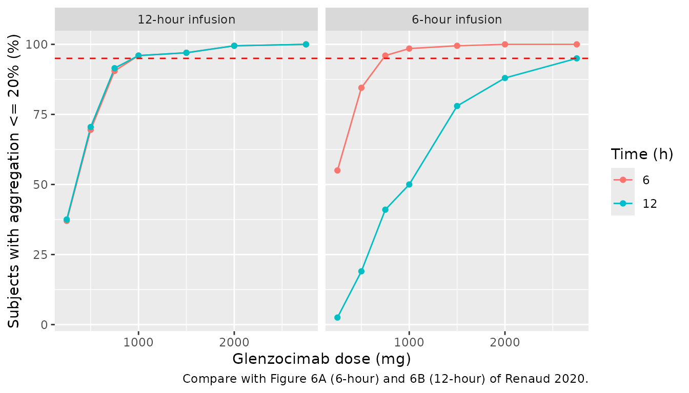
Renaud 2020 simulated 1000 individuals per scenario with IIV and
covariates and without residual error, and reported the percentage
reaching <= 20% aggregation at 6 and 12 hours (Figure 6A, 6B) and the
aggregation remaining at 24 hours (Figure S10). The replication below
uses 200 individuals per dose. The PD model is evaluated through the
PPA prediction column, which excludes residual error.
set.seed(20200902)
rxode2::rxSetSeed(20200902)
n_sc <- 200
scen <- expand.grid(
  dose = c(250, 500, 750, 1000, 1500, 2000, 2750),
  inf_h = c(6, 12),
  stringsAsFactors = FALSE
)
ev_sc <- dplyr::bind_rows(lapply(seq_len(nrow(scen)), function(k) {
  ids <- (k - 1) * n_sc + seq_len(n_sc)
  make_events(ids, scen$dose[k], c(6, 12, 24), inf_h = scen$inf_h[k]) |>
    dplyr::mutate(inf_h = scen$inf_h[k])
}))
ev_sc <- dplyr::left_join(ev_sc, make_cohort(unique(ev_sc$id)), by = "id")

sim_sc <- rxode2::rxSolve(mod, dplyr::select(ev_sc, -inf_h), returnType = "data.frame") |>
  dplyr::mutate(id = as.integer(as.character(id))) |>
  dplyr::left_join(dplyr::distinct(ev_sc, id, inf_h), by = "id")

resp <- sim_sc |>
  dplyr::group_by(inf_h, DOSE, time) |>
  dplyr::summarise(
    pct_le20 = 100 * mean(PPA <= 20),
    median_ppa = median(PPA),
    .groups = "drop"
  )
ggplot(dplyr::filter(resp, time %in% c(6, 12)), aes(DOSE, pct_le20, colour = factor(time))) +
  geom_line() +
  geom_point() +
  geom_hline(yintercept = 95, linetype = "dashed", colour = "red") +
  facet_wrap(~ paste0(inf_h, "-hour infusion")) +
  labs(
    x = "Glenzocimab dose (mg)", y = "Subjects with aggregation <= 20% (%)",
    colour = "Time (h)",
    caption = "Compare with Figure 6A (6-hour) and 6B (12-hour) of Renaud 2020."
  )
resp |>
  dplyr::filter(DOSE %in% c(500, 750, 1000, 2750)) |>
  tidyr::pivot_wider(
    id_cols = c(inf_h, DOSE),
    names_from = time, values_from = c(pct_le20, median_ppa)
  ) |>
  dplyr::select(inf_h, DOSE, pct_le20_6, pct_le20_12, median_ppa_24) |>
  dplyr::rename(
    "Infusion (h)" = inf_h, "Dose (mg)" = DOSE,
    "% <= 20% at 6 h" = pct_le20_6, "% <= 20% at 12 h" = pct_le20_12,
    "Median aggregation at 24 h (%)" = median_ppa_24
  ) |>
knitr::kable(digits = 1)| Infusion (h) | Dose (mg) | % <= 20% at 6 h | % <= 20% at 12 h | Median aggregation at 24 h (%) |
|---|---|---|---|---|
| 6 | 500 | 84.5 | 19.0 | 55.7 |
| 6 | 750 | 96.0 | 41.0 | 39.6 |
| 6 | 1000 | 98.5 | 50.0 | 34.4 |
| 6 | 2750 | 100.0 | 95.0 | 11.0 |
| 12 | 500 | 69.5 | 70.5 | 50.7 |
| 12 | 750 | 90.5 | 91.5 | 36.9 |
| 12 | 1000 | 96.0 | 96.0 | 24.1 |
| 12 | 2750 | 100.0 | 100.0 | 11.5 |
The paper reports, for the 6-hour phase I infusion: about 95% of individuals at <= 20% at 6 hours with 750 mg; nearly 100% at 6 hours and about 60% at 12 hours with 1000 mg; about 2750 mg needed for 95% at 12 hours; and residual aggregation at 24 hours of 55%, 40% and 30% for 500, 750 and 1000 mg (50%, 35% and 25% with a 12-hour infusion).
get_med24 <- function(inf, d) resp$median_ppa[resp$inf_h == inf & resp$DOSE == d & resp$time == 24]
get_pct <- function(inf, d, t) resp$pct_le20[resp$inf_h == inf & resp$DOSE == d & resp$time == t]
med24 <- c(
  get_med24(6, 500), get_med24(6, 750), get_med24(6, 1000),
  get_med24(12, 500), get_med24(12, 750), get_med24(12, 1000)
)
paper24 <- c(55, 40, 30, 50, 35, 25)
knitr::kable(data.frame(
  Infusion = rep(c("6 h", "12 h"), each = 3),
  Dose = rep(c(500, 750, 1000), 2),
  Simulated = round(med24, 1),
  Paper = paper24
))| Infusion | Dose | Simulated | Paper |
|---|---|---|---|
| 6 h | 500 | 55.7 | 55 |
| 6 h | 750 | 39.6 | 40 |
| 6 h | 1000 | 34.4 | 30 |
| 12 h | 500 | 50.7 | 50 |
| 12 h | 750 | 36.9 | 35 |
| 12 h | 1000 | 24.1 | 25 |
stopifnot(
  # Centre of the distribution: robust to which subjects land in the tails.
  all(abs(med24 - paper24) < 10),
  # Near-saturated responder fractions, far from the 20% threshold.
  get_pct(6, 1000, 6) > 85,
  get_pct(6, 2750, 12) > 80
)
The replication lands on the paper’s dose-selection results: 750 mg is the lowest simulated 6-hour-infusion dose with at least 95% of subjects at <= 20% aggregation at 6 hours, 2750 mg is needed for 95% at 12 hours, and a 12-hour infusion reaches 95% at 12 hours with 1000 mg. The simulated 24-hour medians are within 5 percentage points of the paper’s values, which are rounded to 5%; the fraction at <= 20% at 12 hours after 1000 mg (about 50%) is somewhat below the paper’s 60%. The virtual cohort’s covariate distribution is an approximation (see below), and responder fractions near the 20% threshold are sensitive to it.
Assumptions and deviations
- Covariate distribution for the virtual cohort. Renaud 2020 sampled covariates from normal distributions using the phase I means and SDs, truncated at the observed extremes, but printed only medians and ranges (Table 1). The vignette centres each normal on the median with SD = range / 4 and redraws values outside the range.
- 12-hour infusion scheme. The paper does not state how the 12-hour infusion was split. The vignette keeps the phase I loading (25% of the dose in the first 15 minutes) and gives the remaining 75% over 11 h 45 min.
- BLQ handling. The paper fit below-quantification concentrations with the M3 method; this does not affect simulation from the packaged model.
-
Imax covariate range.
Imaxincreases with platelet count; for a platelet count above about 350 x 10^9/L the typicalImaxexceedsBase_PPAand predicted aggregation can fall below 0%, where the logit residual model is undefined. The model is supported for the phase I range of 159-323 x 10^9/L. -
Dose covariate.
DOSEis the total glenzocimab dose (mg) and must be supplied on every record. The authors found no mechanism for the dose-dependent potency; extrapolation beyond 2000 mg (the highest dose studied) relies on this empirical relationship. -
Residual error. Monolix’s
combined1concentration error (SD = a1 + b1 * prediction, Eq. 5) is encoded with rxode2’scombined1(); the aggregation error is a constant SD on the logit of aggregation / 100 (Eq. 6), encoded aslogitNorm(addSd_PPA, 0, 100). -
Observation name. The aggregation endpoint is named
PPAafter the paper’sPPA(t); there is no other percent-aggregation model in the library yet to establish a shared name.