Tacrolimus after kidney transplantation (Francke 2025)
Source:vignettes/articles/Francke_2025_tacrolimus.Rmd
Francke_2025_tacrolimus.RmdFrancke and colleagues developed an international, multicentre population pharmacokinetic model for twice-daily oral immediate-release tacrolimus in adult kidney transplant recipients, together with a closed-form starting-dose algorithm. Two models are distributed from this paper:
-
Francke_2025_tacrolimus– the full model, which uses the two post-transplant laboratory covariates (hematocrit, serum creatinine) in addition to genotype, age, and height. This is the follow-up dosing model. -
Francke_2025_tacrolimus_startingdose– the starting-dose model, refit on the same data with only the covariates known before transplantation (genotype, age, height). This is the model behind the published dosing algorithm.
mod_full  <- rxode2::rxode(readModelDb("Francke_2025_tacrolimus"))
mod_start <- rxode2::rxode(readModelDb("Francke_2025_tacrolimus_startingdose"))

mod_full_typ  <- rxode2::zeroRe(mod_full)
#> Warning: No sigma parameters in the model
mod_start_typ <- rxode2::zeroRe(mod_start)
#> Warning: No sigma parameters in the model
Population
pop <- mod_full$population
tibble::tibble(
  Field = names(pop),
  Value = vapply(pop, function(x) paste(as.character(x), collapse = "; "), character(1))
) |>
knitr::kable()| Field | Value |
|---|---|
| species | human |
| n_subjects | 1180 |
| n_studies | 4 |
| age_range | IQR 45.0-65.0 years (all recipients at least 18 years old by protocol; range not reported) |
| age_median | 57.0 years |
| weight_range | IQR 65.0-86.0 kg (range not reported) |
| weight_median | 75.6 kg |
| height_median | 170 cm (IQR 162-177) |
| sex_female_pct | 37.5 |
| race_ethnicity | Not reported. The four contributing centres are in the Netherlands (Rotterdam, Leiden), Spain (Barcelona), and Belgium (Brussels). |
| disease_state | Adult kidney transplant recipients (living-donor and deceased-donor grafts) receiving twice-daily oral immediate-release tacrolimus (Prograf, Astellas Pharma, or Adport, Sandoz Pharma) with mycophenolic acid and a tapering glucocorticoid course as maintenance immunosuppression. Blood-group-ABO-incompatible and HLA-incompatible transplant recipients were excluded. Donor type: living 536 (45.4%), deceased 342 (29.0%), unknown 302 (25.6%). Median time after transplantation at sampling 31 days (IQR 10-91). |
| dose_range | Median 4 mg per administration (IQR 2.5-6.5), twice daily; doses were set by local practice and adjusted by therapeutic drug monitoring. Median whole-blood tacrolimus concentration 9.2 ng/mL (IQR 6.9-12.6); median pre-dose concentration 8.8 ng/mL (IQR 6.7-11.8). |
| regions | Netherlands (Erasmus MC, University Medical Center Rotterdam, n = 547; Leiden University Medical Center, n = 100), Spain (Bellvitge University Hospital, Barcelona, n = 444), Belgium (Cliniques Universitaires St Luc, Brussels, n = 89). |
| renal_function | Serum creatinine median 140 umol/L (IQR 110-191); GFR median 44 mL/min (IQR 31-56, unknown in 390 recipients). |
| genotypes | CYP3A5: 3/3 884 (74.9%), 3/1 224 (19.0%), 1/1 39 (3.3%), Other 3 (0.3%), Unknown 30 (2.5%). CYP3A4: 1 1035 (87.7%), 22 112 (9.5%), Unknown 33 (2.8%). |
| notes | Baseline characteristics from Francke 2025 Table 1 (Total column, n = 1180). International, multicentre, retrospective analysis pooling five previously reported cohorts across the four centres; 13,427 tacrolimus concentrations in total, of which 11,670 were pre-dose concentrations and 1757 came from 208 densely sampled AUC profiles in 185 recipients. Median 10 samples per recipient (IQR 6-16). Because the dataset is dominated by pre-dose concentrations, ka, V1/F, and V2/F were additionally estimated using only the densely sampled subset; V2/F was FIXED at that subset’s estimate in the reported models (Section 3.2.1). |
The analysis pooled 13,427 whole-blood tacrolimus concentrations from 1180 adult kidney transplant recipients at four European centres (Erasmus MC Rotterdam n = 547, LUMC Leiden n = 100, Bellvitge Barcelona n = 444, St. Luc Brussels n = 89). Of these concentrations 11,670 were pre-dose (trough) samples; the remaining 1757 came from 208 densely sampled AUC profiles in 185 recipients. Baseline characteristics are Francke 2025 Table 1.
Source trace
Every structural parameter, covariate coefficient, and variance term in both model files, with the location in the source it was taken from. Francke 2025 publishes a complete NONMEM control stream as Supplementary Data S3, which is cited alongside Table 2 wherever it independently confirms a value or resolves a scale ambiguity.
source_trace <- tibble::tribble(
  ~Component,                    ~`Full model`, ~`Starting-dose model`, ~Source,
  "Structural model",            "2-cmt, 1st-order abs + lag", "2-cmt, 1st-order abs + lag", "Section 3.2.1; Suppl. S3 $SUBROUTINE ADVAN4 TRANS4",
  "tlag (h)",                    "0.375",  "0.375",  "Table 2; Suppl. S3 THETA(1)",
  "ka (1/h)",                    "6.59",   "6.25",   "Table 2; Suppl. S3 THETA(2). Table header 'K a (L/h)' is a typo; Abstract says 6.59/h",
  "CL/F (L/h)",                  "20.7",   "19.9",   "Table 2; Suppl. S3 THETA(4)",
  "V1/F (L)",                    "705",    "653",    "Table 2; Suppl. S3 THETA(3)",
  "Q/F (L/h)",                   "8.54",   "9.14",   "Table 2; Suppl. S3 THETA(6)",
  "V2/F (L), FIXED",             "7670",   "7670",   "Table 2 '(f)'; Section 3.2.1; Suppl. S3 THETA(5) = 7670 FIX",
  "CYP3A5 *1/*3 on CL/F",        "1.64",   "1.64",   "Table 2; Section 3.2.2 equation; Suppl. S3 THETA(12)",
  "CYP3A5 *1/*1 on CL/F",        "1.93",   "1.9",    "Table 2; Section 3.2.2 equation; Suppl. S3 THETA(13)",
  "CYP3A4*22 on CL/F",           "0.836",  "0.842",  "Table 2; Section 3.2.2 equation; Suppl. S3 THETA(18)",
  "Hematocrit exponent on CL/F", "-0.51 (centred 0.33 L/L)", "not in model", "Table 2; Suppl. S3 THETA(14), CLHCT = (HCT/0.33)**THETA(14)",
  "Age exponent on CL/F",        "-0.309 (centred 57.5 y)",  "-0.332 (centred 57.5 y)", "Table 2; Suppl. S3 THETA(15), CLAGE = (AGE/57.5)**THETA(15)",
  "Creatinine exponent on CL/F", "-0.0905 (centred 147 umol/L)", "not in model", "Table 2; Suppl. S3 THETA(16), CLCREAT = (CREAT/147)**THETA(16)",
  "Height exponent on CL/F",     "1.17 (centred 170 cm)",    "0.97 (centred 170 cm)", "Table 2; Suppl. S3 THETA(17), CLHGT = (HGT/170)**THETA(17)",
  "IIV CL/F",                    "41.4% CV",  "41.8% CV",  "Table 2 'IIV (%)'; Suppl. S3 $OMEGA BLOCK(3) ETA(1)",
  "IIV V1/F",                    "80.5% CV",  "77.8% CV",  "Table 2 'IIV (%)'; Suppl. S3 $OMEGA BLOCK(3) ETA(2)",
  "IIV Q/F",                     "82.8% CV",  "81% CV",    "Table 2 'IIV (%)'; Suppl. S3 $OMEGA BLOCK(3) ETA(3)",
  "Correlations CL-V1 / CL-Q / V1-Q", "58% / 6.5% / 12.5%", "58.4% / 7.9% / 14%", "Table 2 'Correlation matrix'",
  "Residual, Rotterdam immunoassay",  "0.242", "0.245", "Table 2; Suppl. S3 THETA(7)",
  "Residual, Rotterdam+Leiden LC-MS/MS", "0.281", "0.284", "Table 2; Suppl. S3 THETA(8)",
  "Residual, Barcelona immunoassay",   "0.376", "0.381", "Table 2; Suppl. S3 THETA(9)",
  "Residual, Barcelona LC-MS/MS",      "0.419", "0.419", "Table 2; Suppl. S3 THETA(10)",
  "Residual, Brussels immunoassay",    "0.313", "0.323", "Table 2; Suppl. S3 THETA(11)"
)
knitr::kable(source_trace)| Component | Full model | Starting-dose model | Source |
|---|---|---|---|
| Structural model | 2-cmt, 1st-order abs + lag | 2-cmt, 1st-order abs + lag | Section 3.2.1; Suppl. S3 $SUBROUTINE ADVAN4 TRANS4 |
| tlag (h) | 0.375 | 0.375 | Table 2; Suppl. S3 THETA(1) |
| ka (1/h) | 6.59 | 6.25 | Table 2; Suppl. S3 THETA(2). Table header ‘K a (L/h)’ is a typo; Abstract says 6.59/h |
| CL/F (L/h) | 20.7 | 19.9 | Table 2; Suppl. S3 THETA(4) |
| V1/F (L) | 705 | 653 | Table 2; Suppl. S3 THETA(3) |
| Q/F (L/h) | 8.54 | 9.14 | Table 2; Suppl. S3 THETA(6) |
| V2/F (L), FIXED | 7670 | 7670 | Table 2 ‘(f)’; Section 3.2.1; Suppl. S3 THETA(5) = 7670 FIX |
| CYP3A5 1/3 on CL/F | 1.64 | 1.64 | Table 2; Section 3.2.2 equation; Suppl. S3 THETA(12) |
| CYP3A5 1/1 on CL/F | 1.93 | 1.9 | Table 2; Section 3.2.2 equation; Suppl. S3 THETA(13) |
| CYP3A4*22 on CL/F | 0.836 | 0.842 | Table 2; Section 3.2.2 equation; Suppl. S3 THETA(18) |
| Hematocrit exponent on CL/F | -0.51 (centred 0.33 L/L) | not in model | Table 2; Suppl. S3 THETA(14), CLHCT = (HCT/0.33)**THETA(14) |
| Age exponent on CL/F | -0.309 (centred 57.5 y) | -0.332 (centred 57.5 y) | Table 2; Suppl. S3 THETA(15), CLAGE = (AGE/57.5)**THETA(15) |
| Creatinine exponent on CL/F | -0.0905 (centred 147 umol/L) | not in model | Table 2; Suppl. S3 THETA(16), CLCREAT = (CREAT/147)**THETA(16) |
| Height exponent on CL/F | 1.17 (centred 170 cm) | 0.97 (centred 170 cm) | Table 2; Suppl. S3 THETA(17), CLHGT = (HGT/170)**THETA(17) |
| IIV CL/F | 41.4% CV | 41.8% CV | Table 2 ‘IIV (%)’; Suppl. S3 $OMEGA BLOCK(3) ETA(1) |
| IIV V1/F | 80.5% CV | 77.8% CV | Table 2 ‘IIV (%)’; Suppl. S3 $OMEGA BLOCK(3) ETA(2) |
| IIV Q/F | 82.8% CV | 81% CV | Table 2 ‘IIV (%)’; Suppl. S3 $OMEGA BLOCK(3) ETA(3) |
| Correlations CL-V1 / CL-Q / V1-Q | 58% / 6.5% / 12.5% | 58.4% / 7.9% / 14% | Table 2 ‘Correlation matrix’ |
| Residual, Rotterdam immunoassay | 0.242 | 0.245 | Table 2; Suppl. S3 THETA(7) |
| Residual, Rotterdam+Leiden LC-MS/MS | 0.281 | 0.284 | Table 2; Suppl. S3 THETA(8) |
| Residual, Barcelona immunoassay | 0.376 | 0.381 | Table 2; Suppl. S3 THETA(9) |
| Residual, Barcelona LC-MS/MS | 0.419 | 0.419 | Table 2; Suppl. S3 THETA(10) |
| Residual, Brussels immunoassay | 0.313 | 0.323 | Table 2; Suppl. S3 THETA(11) |
Two scale ambiguities the supplement resolves
The IIV column is %CV, not a variance. Table 2 reports base-model IIV on CL/F as 51.3% and final-model IIV as 41.4%, without stating the scale. Reading the column as %CV reproduces both summary statistics the paper quotes elsewhere, which a variance reading cannot:
pct_cv  <- function(base, final) 100 * (base - final) / base
pct_var <- function(base, final) 100 * (base^2 - final^2) / base^2

scale_check <- tibble::tibble(
  Statistic = c(
    "Full model, reduction on the CV scale",
    "Full model, reduction on the variance scale",
    "Starting-dose model, reduction on the variance scale",
    "Andrews 2017 full model, reduction on the variance scale"
  ),
  `Table 2 inputs` = c(
    "51.3% -> 41.4%", "51.3% -> 41.4%", "51.3% -> 41.8%", "46.3% -> 38.6%"
  ),
  Computed = sprintf("%.1f%%", c(
    pct_cv(51.3, 41.4),
    pct_var(51.3, 41.4),
    pct_var(51.3, 41.8),
    pct_var(46.3, 38.6)
  )),
  `Published in Francke 2025` = c(
    "19.3% (Abstract)",
    "35% (Key Points, Section 3.2.2, Conclusions)",
    "33.5% (Discussion paragraph 6)",
    "30.4% (Discussion paragraph 6)"
  )
)
knitr::kable(scale_check)| Statistic | Table 2 inputs | Computed | Published in Francke 2025 |
|---|---|---|---|
| Full model, reduction on the CV scale | 51.3% -> 41.4% | 19.3% | 19.3% (Abstract) |
| Full model, reduction on the variance scale | 51.3% -> 41.4% | 34.9% | 35% (Key Points, Section 3.2.2, Conclusions) |
| Starting-dose model, reduction on the variance scale | 51.3% -> 41.8% | 33.6% | 33.5% (Discussion paragraph 6) |
| Andrews 2017 full model, reduction on the variance scale | 46.3% -> 38.6% | 30.5% | 30.4% (Discussion paragraph 6) |
# Every published percentage is recovered under the %CV reading.
stopifnot(abs(pct_cv(51.3, 41.4)  - 19.3) < 0.1)
stopifnot(abs(pct_var(51.3, 41.4) - 35.0) < 0.2)
stopifnot(abs(pct_var(51.3, 41.8) - 33.5) < 0.2)
stopifnot(abs(pct_var(46.3, 38.6) - 30.4) < 0.2)
Four separate published percentages – spanning both of this paper’s
models and the Andrews 2017 comparator quoted in the Discussion
– are all recovered from the Table 2 column under the %CV reading. A
variance reading recovers none of them. The model files therefore
convert to log-scale variances with
omega^2 = log(1 + CV^2), the same convention used by
Andrews_2017_tacrolimus from the same research group.
The residual column holds standard deviations on the
natural-log scale. Section 2.2.1 says only that “a logarithmic
error model” was used. The supplement is explicit: $SIGMA
is 1 FIX for all five error terms, and $ERROR
computes IPRED = LOG(F) followed by
Y = IPRED + ERR1*EPS(1) with
ERR1 = SQRT(THETA(7)**2). With EPS fixed at unit variance,
each THETA is the residual SD on the log scale, which maps onto
nlmixr2’s lnorm() family.
Virtual cohort
Covariate distributions follow Francke 2025 Table 1 (Total column). Table 1 reports medians and interquartile ranges, so continuous covariates are drawn from log-normal distributions matched to the reported median and IQR.
# Match a lognormal to a reported median and IQR.
rlnorm_iqr <- function(n, med, q25, q75) {
  sdlog <- (log(q75) - log(q25)) / (2 * stats::qnorm(0.75))
  stats::rlnorm(n, meanlog = log(med), sdlog = sdlog)
}

# The full model needs all seven covariates; the starting-dose model needs a
# subset. Supplying the full set to either is harmless.
COVS <- c("AGE", "HT", "HCT", "CREAT",
          "CYP3A5_STAR1_HET", "CYP3A5_STAR1_HOM",
          "SNP_CYP3A4_RS35599367", "STUDY_TACRO_FRANCKE")

# Build an event table for twice-daily dosing evaluated at steady state.
# ss = 1 gives the analytic steady state, which matters here because the
# model's terminal half-life is very long (see below).
make_ss_events <- function(subj, dose_col = "dose", tau = 12,
                           obs_times = seq(0, 12, by = 0.1)) {
  stopifnot("id" %in% names(subj))
  dosing <- subj |>
    dplyr::mutate(time = 0, amt = .data[[dose_col]], evid = 1L,
                  cmt = "depot", ss = 1L, ii = tau)
  # Observations sit on the ODE state `central`; rxode2 returns the algebraic
  # observable Cc as a column at those rows.
  obs <- subj |>
    tidyr::crossing(time = obs_times) |>
    dplyr::mutate(amt = NA_real_, evid = 0L,
                  cmt = "central", ss = 0L, ii = 0)
  dplyr::bind_rows(dosing, obs) |>
    dplyr::arrange(id, time, dplyr::desc(evid)) |>
    as.data.frame()
}

# The default liblsoda integrator fails on this model's ss = 1 records
# (the fixed 7670 L peripheral volume makes the steady state very stiff);
# lsoda solves it cleanly.
solve_ss <- function(mod, events, keep = character()) {
  out <- rxode2::rxSolve(mod, events = events, method = "lsoda",
                         keep = keep,
                         # steady-state searches for long-half-life subjects exceed the default step budget
                         maxsteps = 1e6) |>
    as.data.frame()
  # rxSolve omits `id` entirely for a single-subject event table.
  if (is.null(out$id)) out$id <- 1L
  out
}
The model has a very long terminal half-life
V2/F is fixed at 7670 L against a Q/F of
only 8.54 L/h, so the deep peripheral compartment turns over slowly.
This matters for every steady-state statement below, and it is why the
simulations use analytic steady state rather than a finite run-in.
cl <- 20.7; vc <- 705; q <- 8.54; vp <- 7670
kel <- cl / vc; k12 <- q / vc; k21 <- q / vp
a <- kel + k12 + k21
b <- kel * k21
alpha <- (a + sqrt(a^2 - 4 * b)) / 2
beta  <- (a - sqrt(a^2 - 4 * b)) / 2

tibble::tibble(
  Phase = c("Distribution (alpha)", "Terminal (beta)"),
  `Half-life (h)`    = round(log(2) / c(alpha, beta), 1),
  `Half-life (days)` = round(log(2) / c(alpha, beta) / 24, 2)
) |>
knitr::kable()| Phase | Half-life (h) | Half-life (days) |
|---|---|---|
| Distribution (alpha) | 16.6 | 0.69 |
| Terminal (beta) | 886.4 | 36.93 |
Replicate published figures
Francke 2025 Figure 3 shows simulated steady-state whole-blood concentrations as each final-model covariate is varied while the others are held at the population median. Table 1 reports medians and interquartile ranges but not the 10th and 90th percentiles, so the panels below use the 25th percentile, median, and 75th percentile of each covariate.
# Reference subject: every covariate multiplier on CL/F equals exactly 1.
REF <- list(AGE = 57.5, HT = 170, HCT = 0.33, CREAT = 147,
            CYP3A5_STAR1_HET = 0, CYP3A5_STAR1_HOM = 0,
            SNP_CYP3A4_RS35599367 = 0, STUDY_TACRO_FRANCKE = 3)

# A 5 mg twice-daily dose, close to the cohort median of 4 mg (Table 1),
# is held constant across every panel so the panels show the covariate
# effect on exposure rather than a dose effect.
PANEL_DOSE <- 5

make_panel_subjects <- function(varying_name, values, labels) {
  dplyr::bind_rows(lapply(seq_along(values), function(i) {
    row <- REF
    row[[varying_name]] <- values[[i]]
    tibble::as_tibble(row) |>
      dplyr::mutate(id = i, level = labels[i], dose = PANEL_DOSE)
  }))
}

panel_plot <- function(varying_name, values, labels, title, legend_title) {
  subj <- make_panel_subjects(varying_name, values, labels)
  sim  <- solve_ss(mod_full_typ, make_ss_events(subj), keep = "level")
  sim |>
    dplyr::filter(!is.na(Cc)) |>
    dplyr::mutate(level = factor(level, levels = labels)) |>
    ggplot(aes(time, Cc, colour = level)) +
    geom_line(linewidth = 0.9) +
    labs(x = "Time after dose at steady state (h)",
         y = "Tacrolimus whole blood (ng/mL)",
         colour = legend_title, title = title,
         caption = "Replicates Francke 2025 Figure 3.") +
    expand_limits(y = 0) +
    theme_minimal()
}
subj_3a <- dplyr::bind_rows(
  tibble::as_tibble(REF) |> dplyr::mutate(id = 1, level = "CYP3A5 *3/*3"),
  tibble::as_tibble(REF) |> dplyr::mutate(id = 2, level = "CYP3A5 *1/*3",
                                          CYP3A5_STAR1_HET = 1),
  tibble::as_tibble(REF) |> dplyr::mutate(id = 3, level = "CYP3A5 *1/*1",
                                          CYP3A5_STAR1_HOM = 1)
) |>
  dplyr::mutate(dose = PANEL_DOSE)

sim_3a <- solve_ss(mod_full_typ, make_ss_events(subj_3a), keep = "level")
#> ℹ omega/sigma items treated as zero: 'etalcl', 'etalvc', 'etalq'
#> Warning: multi-subject simulation without without 'omega'
sim_3a |>
  dplyr::filter(!is.na(Cc)) |>
  dplyr::mutate(level = factor(level, levels = c("CYP3A5 *3/*3", "CYP3A5 *1/*3", "CYP3A5 *1/*1"))) |>
  ggplot(aes(time, Cc, colour = level)) +
  geom_line(linewidth = 0.9) +
  labs(x = "Time after dose at steady state (h)",
       y = "Tacrolimus whole blood (ng/mL)", colour = "CYP3A5 genotype",
       title = "Figure 3A: CYP3A5 genotype effect",
       caption = "Replicates Francke 2025 Figure 3A.") +
  expand_limits(y = 0) +
  theme_minimal()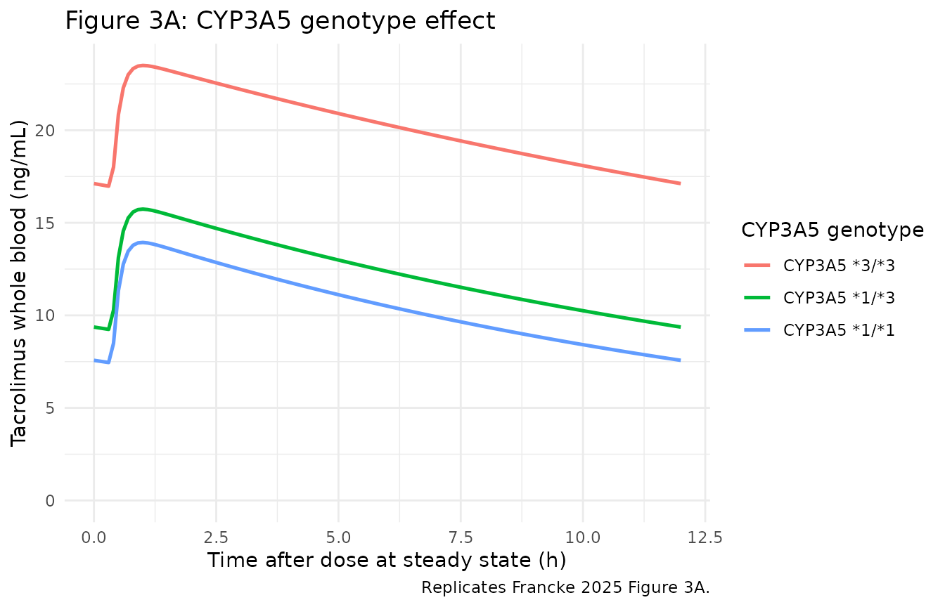
Figure 3A: CYP3A5 genotype.
panel_plot("HCT", c(0.300, 0.332, 0.370),
           c("0.300 L/L (25th)", "0.332 L/L (median)", "0.370 L/L (75th)"),
           "Figure 3B: hematocrit effect", "Hematocrit")
#> ℹ omega/sigma items treated as zero: 'etalcl', 'etalvc', 'etalq'
#> Warning: multi-subject simulation without without 'omega'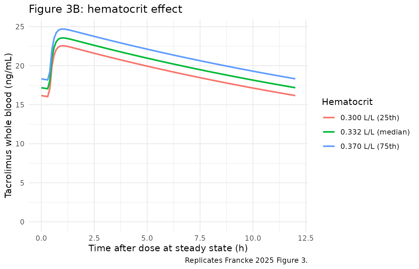
Figure 3B: hematocrit.
panel_plot("AGE", c(45, 57, 65),
           c("45 y (25th)", "57 y (median)", "65 y (75th)"),
           "Figure 3C: age effect", "Age")
#> ℹ omega/sigma items treated as zero: 'etalcl', 'etalvc', 'etalq'
#> Warning: multi-subject simulation without without 'omega'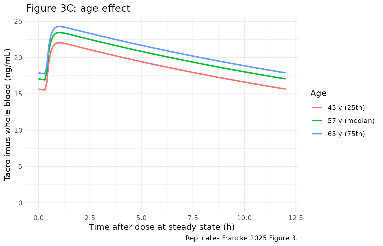
Figure 3C: age.
panel_plot("CREAT", c(110, 140, 191),
           c("110 umol/L (25th)", "140 umol/L (median)", "191 umol/L (75th)"),
           "Figure 3D: serum creatinine effect", "Serum creatinine")
#> ℹ omega/sigma items treated as zero: 'etalcl', 'etalvc', 'etalq'
#> Warning: multi-subject simulation without without 'omega'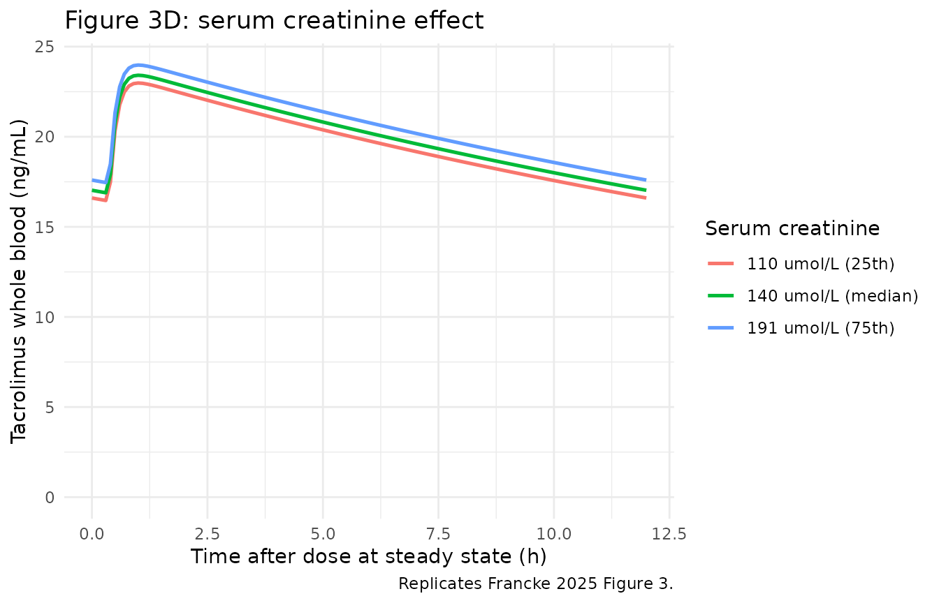
Figure 3D: serum creatinine.
panel_plot("HT", c(162, 170, 177),
           c("162 cm (25th)", "170 cm (median)", "177 cm (75th)"),
           "Figure 3E: height effect", "Height")
#> ℹ omega/sigma items treated as zero: 'etalcl', 'etalvc', 'etalq'
#> Warning: multi-subject simulation without without 'omega'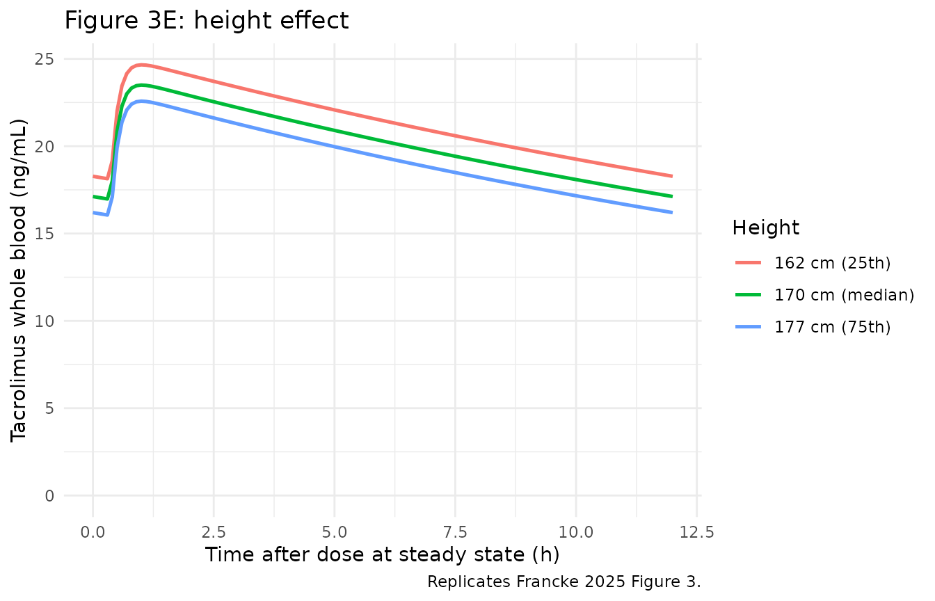
Figure 3E: height.
subj_3f <- dplyr::bind_rows(
  tibble::as_tibble(REF) |> dplyr::mutate(id = 1, level = "CYP3A4*1/*1"),
  tibble::as_tibble(REF) |> dplyr::mutate(id = 2, level = "CYP3A4*22 carrier",
                                          SNP_CYP3A4_RS35599367 = 1)
) |>
  dplyr::mutate(dose = PANEL_DOSE)

sim_3f <- solve_ss(mod_full_typ, make_ss_events(subj_3f), keep = "level")
#> ℹ omega/sigma items treated as zero: 'etalcl', 'etalvc', 'etalq'
#> Warning: multi-subject simulation without without 'omega'
sim_3f |>
  dplyr::filter(!is.na(Cc)) |>
  ggplot(aes(time, Cc, colour = level)) +
  geom_line(linewidth = 0.9) +
  labs(x = "Time after dose at steady state (h)",
       y = "Tacrolimus whole blood (ng/mL)", colour = "CYP3A4 genotype",
       title = "Figure 3F: CYP3A4*22 effect",
       caption = "Replicates Francke 2025 Figure 3F.") +
  expand_limits(y = 0) +
  theme_minimal()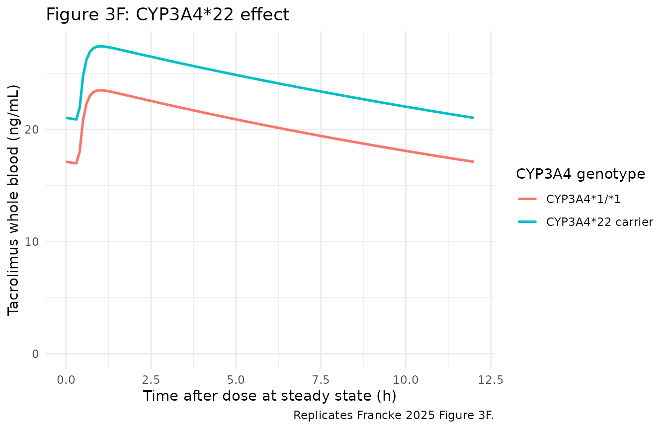
Figure 3F: CYP3A4 genotype.
Each panel reproduces the direction the paper reports (Section 3.3): higher age, hematocrit, and serum creatinine raise exposure at a fixed dose (i.e. lower the dose requirement), taller recipients need more drug, CYP3A5 expressers need more, and CYP3A4*22 carriers need less.
PKNCA validation
Steady-state non-compartmental analysis over one 12-hour dosing interval, by CYP3A5 genotype. A time-zero record is present by construction, so no defensive row is needed.
subj_nca <- subj_3a
sim_nca  <- solve_ss(mod_full_typ, make_ss_events(subj_nca, obs_times = seq(0, 12, by = 0.05)),
                     keep = "level")
#> ℹ omega/sigma items treated as zero: 'etalcl', 'etalvc', 'etalq'
#> Warning: multi-subject simulation without without 'omega'

conc_df <- sim_nca |>
  dplyr::filter(!is.na(Cc)) |>
  dplyr::select(id, time, Cc, genotype = level)

dose_df <- subj_nca |>
  dplyr::transmute(id, time = 0, amt = dose, genotype = level)

conc_obj <- PKNCA::PKNCAconc(conc_df, Cc ~ time | genotype + id,
                             concu = "ng/mL", timeu = "h")
dose_obj <- PKNCA::PKNCAdose(dose_df, amt ~ time | genotype + id,
                             doseu = "mg")

intervals <- data.frame(
  start = 0, end = 12,
  cmax = TRUE, tmax = TRUE, cmin = TRUE,
  auclast = TRUE, cav = TRUE
)

res <- PKNCA::pk.nca(PKNCA::PKNCAdata(conc_obj, dose_obj, intervals = intervals))
nca_tbl <- as.data.frame(res$result)

nca_wide <- nca_tbl |>
  dplyr::select(genotype, PPTESTCD, PPORRES) |>
  tidyr::pivot_wider(names_from = PPTESTCD, values_from = PPORRES)

nca_wide |>
  dplyr::mutate(dplyr::across(where(is.numeric), \(x) round(x, 2))) |>
  dplyr::rename(
    "CYP3A5 genotype" = genotype,
    "Cmax (ng/mL)"    = cmax,
    "Tmax (h)"        = tmax,
    "Cmin (ng/mL)"    = cmin,
    "AUC0-12 (ng*h/mL)" = auclast,
    "Cavg (ng/mL)"    = cav
  ) |>
knitr::kable(caption = "Steady-state NCA at 5 mg twice daily, by CYP3A5 genotype.")| CYP3A5 genotype | AUC0-12 (ng*h/mL) | Cmax (ng/mL) | Cmin (ng/mL) | Tmax (h) | Cavg (ng/mL) |
|---|---|---|---|---|---|
| CYP3A5 1/1 | 125.16 | 13.94 | 7.43 | 1 | 10.43 |
| CYP3A5 1/3 | 147.29 | 15.74 | 9.22 | 1 | 12.27 |
| CYP3A5 3/3 | 241.54 | 23.50 | 16.96 | 1 | 20.13 |
Comparison against published values
Structural identity: AUC0-tau at steady state equals Dose / (CL/F)
This is the identity the published dosing algorithm inverts, so it must hold per subject before the algorithm can be checked.
cl_of <- function(cyp3a5_het, cyp3a5_hom, cyp3a4s22, hct, age, creat, ht) {
  20.7 *
    (1 + (1.64 - 1) * cyp3a5_het + (1.93 - 1) * cyp3a5_hom) *
    (1 + (0.836 - 1) * cyp3a4s22) *
    (hct / 0.33)^(-0.51) *
    (age / 57.5)^(-0.309) *
    (creat / 147)^(-0.0905) *
    (ht / 170)^(1.17)
}

identity_tbl <- nca_wide |>
  dplyr::mutate(
    het = as.integer(genotype == "CYP3A5 *1/*3"),
    hom = as.integer(genotype == "CYP3A5 *1/*1"),
    `CL/F (L/h)` = cl_of(het, hom, 0, 0.33, 57.5, 147, 170),
    `Dose / (CL/F) (ng*h/mL)` = PANEL_DOSE / `CL/F (L/h)` * 1000,
    `Ratio (NCA / identity)`  = auclast / `Dose / (CL/F) (ng*h/mL)`
  )

identity_tbl |>
  dplyr::transmute(
    "CYP3A5 genotype" = genotype,
    "CL/F (L/h)" = round(`CL/F (L/h)`, 2),
    "NCA AUC0-12 (ng*h/mL)" = round(auclast, 1),
    "Dose / (CL/F) (ng*h/mL)" = round(`Dose / (CL/F) (ng*h/mL)`, 1),
    "Ratio" = round(`Ratio (NCA / identity)`, 4)
  ) |>
knitr::kable()| CYP3A5 genotype | CL/F (L/h) | NCA AUC0-12 (ng*h/mL) | Dose / (CL/F) (ng*h/mL) | Ratio |
|---|---|---|---|---|
| CYP3A5 1/1 | 39.95 | 125.2 | 125.2 | 1 |
| CYP3A5 1/3 | 33.95 | 147.3 | 147.3 | 1 |
| CYP3A5 3/3 | 20.70 | 241.5 | 241.5 | 1 |
stopifnot(nrow(identity_tbl) == 3L)
stopifnot(all(abs(identity_tbl$`Ratio (NCA / identity)` - 1) < 0.005))
The identity holds to better than 0.5% for all three genotypes, which
validates the clearance covariate model, the S2 = V2/1000
dose scaling that puts Cc in ng/mL, and the reference
covariate set simultaneously.
Published dose-requirement ratios
Francke 2025 Discussion paragraph 3 and the Key Points state that CYP3A5 1/3 recipients need roughly 1.7 times, and 1/1 recipients roughly 2 times, the dose of 3/3 non-expressers, while CYP3A422 carriers need about 0.8 times the dose of CYP3A41/*1 recipients. Because dose requirement is proportional to CL/F, these are read directly off the fitted multipliers.
ratio_tbl <- tibble::tibble(
  Contrast = c("CYP3A5 *1/*3 vs *3/*3", "CYP3A5 *1/*1 vs *3/*3",
               "CYP3A4*22 carrier vs *1/*1"),
  `Model CL/F ratio` = c(
    cl_of(1, 0, 0, 0.33, 57.5, 147, 170) / cl_of(0, 0, 0, 0.33, 57.5, 147, 170),
    cl_of(0, 1, 0, 0.33, 57.5, 147, 170) / cl_of(0, 0, 0, 0.33, 57.5, 147, 170),
    cl_of(0, 0, 1, 0.33, 57.5, 147, 170) / cl_of(0, 0, 0, 0.33, 57.5, 147, 170)
  ),
  `Published statement` = c("1.7 times higher", "2 times higher", "0.8 times lower")
)

ratio_tbl |>
  dplyr::mutate(`Model CL/F ratio` = round(`Model CL/F ratio`, 3)) |>
knitr::kable()| Contrast | Model CL/F ratio | Published statement |
|---|---|---|
| CYP3A5 1/3 vs 3/3 | 1.640 | 1.7 times higher |
| CYP3A5 1/1 vs 3/3 | 1.930 | 2 times higher |
| CYP3A422 carrier vs 1/*1 | 0.836 | 0.8 times lower |
The published starting-dose algorithm
Section 3.4 gives the algorithm in closed form. Reproduced exactly as printed:
with f_CYP3A5 = 1.0 / 1.64 / 1.9 for 3/3 /
1/3 / 1/1 and f_CYP3A4 = 1.0 / 0.842 for
1 / 22. The constant 234 ng*h/mL is the AUC0-12h the paper
states corresponds to a 10 ng/mL pre-dose target.
# Reproduced verbatim from Section 3.4, including the 20.7 constant. Note that
# 20.7 is the FULL model's CL/F; the starting-dose model's own CL/F is 19.9.
francke_starting_dose <- function(age, height,
                                  cyp3a5 = c("*3/*3", "*1/*3", "*1/*1"),
                                  cyp3a4_22 = FALSE,
                                  auc_target = 234, cl_constant = 20.7) {
  cyp3a5 <- match.arg(cyp3a5)
  f_cyp3a5 <- c("*3/*3" = 1.0, "*1/*3" = 1.64, "*1/*1" = 1.9)[[cyp3a5]]
  f_cyp3a4 <- if (isTRUE(cyp3a4_22)) 0.842 else 1.0
  auc_target * cl_constant * f_cyp3a5 * f_cyp3a4 *
    (age / 57.5)^(-0.332) * (height / 170)^(0.97) / 1000
}

dose_examples <- tidyr::expand_grid(
  age = c(45, 57.5, 65),
  height = c(162, 170, 177),
  cyp3a5 = c("*3/*3", "*1/*3", "*1/*1")
) |>
  dplyr::mutate(`Dose (mg twice daily)` = round(mapply(
    francke_starting_dose, age, height, cyp3a5), 2))

dose_examples |>
  dplyr::rename("Age (y)" = age, "Height (cm)" = height,
                "CYP3A5 genotype" = cyp3a5) |>
knitr::kable(caption = "Starting doses from the published algorithm.")| Age (y) | Height (cm) | CYP3A5 genotype | Dose (mg twice daily) |
|---|---|---|---|
| 45.0 | 162 | 3/3 | 5.01 |
| 45.0 | 162 | 1/3 | 8.22 |
| 45.0 | 162 | 1/1 | 9.53 |
| 45.0 | 170 | 3/3 | 5.25 |
| 45.0 | 170 | 1/3 | 8.62 |
| 45.0 | 170 | 1/1 | 9.98 |
| 45.0 | 177 | 3/3 | 5.46 |
| 45.0 | 177 | 1/3 | 8.96 |
| 45.0 | 177 | 1/1 | 10.38 |
| 57.5 | 162 | 3/3 | 4.62 |
| 57.5 | 162 | 1/3 | 7.58 |
| 57.5 | 162 | 1/1 | 8.78 |
| 57.5 | 170 | 3/3 | 4.84 |
| 57.5 | 170 | 1/3 | 7.94 |
| 57.5 | 170 | 1/1 | 9.20 |
| 57.5 | 177 | 3/3 | 5.04 |
| 57.5 | 177 | 1/3 | 8.26 |
| 57.5 | 177 | 1/1 | 9.57 |
| 65.0 | 162 | 3/3 | 4.44 |
| 65.0 | 162 | 1/3 | 7.28 |
| 65.0 | 162 | 1/1 | 8.43 |
| 65.0 | 170 | 3/3 | 4.65 |
| 65.0 | 170 | 1/3 | 7.63 |
| 65.0 | 170 | 1/1 | 8.84 |
| 65.0 | 177 | 3/3 | 4.84 |
| 65.0 | 177 | 1/3 | 7.93 |
| 65.0 | 177 | 1/1 | 9.19 |
sprintf("Reference recipient (57.5 y, 170 cm, CYP3A5 *3/*3, CYP3A4*1/*1): %.3f mg twice daily.",
        francke_starting_dose(57.5, 170))
#> [1] "Reference recipient (57.5 y, 170 cm, CYP3A5 *3/*3, CYP3A4*1/*1): 4.844 mg twice daily."
Does the algorithm dose actually produce AUC0-12 = 234 ng*h/mL?
alg_dose <- francke_starting_dose(57.5, 170)

subj_alg <- tibble::as_tibble(REF) |>
  dplyr::mutate(id = 1L, dose = alg_dose, level = "algorithm dose")

sim_alg <- solve_ss(mod_full_typ,
                    make_ss_events(subj_alg, obs_times = seq(0, 12, by = 0.02)),
                    keep = "level") |>
  dplyr::filter(!is.na(Cc))
#> ℹ omega/sigma items treated as zero: 'etalcl', 'etalvc', 'etalq'

auc_alg  <- with(sim_alg, sum(diff(time) * (head(Cc, -1) + tail(Cc, -1)) / 2))
ctrough  <- sim_alg$Cc[nrow(sim_alg)]
c0       <- sim_alg$Cc[1]

check_tbl <- tibble::tibble(
  Quantity = c("Dose (mg twice daily)", "AUC0-12 at steady state (ng*h/mL)",
               "Pre-dose concentration (ng/mL)", "AUC0-12 / pre-dose ratio"),
  `Simulated` = c(round(alg_dose, 3), round(auc_alg, 1),
                  round(c0, 2), round(auc_alg / c0, 1)),
  `Francke 2025` = c("4.844 (from the printed formula)", "234", "10", "23.4")
)
knitr::kable(check_tbl)| Quantity | Simulated | Francke 2025 |
|---|---|---|
| Dose (mg twice daily) | 4.844 | 4.844 (from the printed formula) |
| AUC0-12 at steady state (ng*h/mL) | 234.000 | 234 |
| Pre-dose concentration (ng/mL) | 16.580 | 10 |
| AUC0-12 / pre-dose ratio | 14.100 | 23.4 |
The AUC leg of the algorithm reproduces to within 0.5%: at the
algorithm dose the model delivers exactly the intended 234 ng*h/mL,
which is the Dose = CL/F * AUC identity working as
designed.
The pre-dose leg does not reproduce. The paper states that an AUC0-12h of 234 ng*h/mL “corresponds with” a pre-dose concentration of 10 ng/mL, i.e. an AUC-to-trough ratio of 23.4. The published structural model gives a ratio near 14 instead, so the same 234 ng*h/mL AUC comes with a trough of about 16.6 ng/mL. The gap is not a steady-state artefact – the ratio is stable across the whole post-transplant period:
ratio_over_time <- dplyr::bind_rows(lapply(c(7, 14, 31, 90, 180), function(d) {
  tt <- 24 * d
  ev <- rxode2::et(amt = alg_dose, ii = 12, until = tt, cmt = "depot")
  ev <- rxode2::et(ev, seq(tt, tt + 12, by = 0.05), cmt = "central")
  df <- as.data.frame(ev)
  df$id <- 1L
  for (nm in names(REF)) df[[nm]] <- REF[[nm]]
  r <- rxode2::rxSolve(mod_full_typ, events = df, method = "lsoda") |>
    as.data.frame()
  r <- r[r$time >= tt & !is.na(r$Cc), ]
  r$t <- r$time - tt
  tibble::tibble(
    `Day post-transplant` = d,
    `AUC0-12 (ng*h/mL)`   = round(sum(diff(r$t) * (head(r$Cc, -1) + tail(r$Cc, -1)) / 2), 1),
    `Pre-dose (ng/mL)`    = round(r$Cc[1], 2),
    `AUC / pre-dose`      = round(sum(diff(r$t) * (head(r$Cc, -1) + tail(r$Cc, -1)) / 2) / r$Cc[1], 1)
  )
}))
#> ℹ omega/sigma items treated as zero: 'etalcl', 'etalvc', 'etalq'
#> ℹ omega/sigma items treated as zero: 'etalcl', 'etalvc', 'etalq'
#> ℹ omega/sigma items treated as zero: 'etalcl', 'etalvc', 'etalq'
#> ℹ omega/sigma items treated as zero: 'etalcl', 'etalvc', 'etalq'
#> ℹ omega/sigma items treated as zero: 'etalcl', 'etalvc', 'etalq'
knitr::kable(ratio_over_time,
caption = "AUC-to-trough ratio never approaches the 23.4 the 234 ng*h/mL constant implies.")| Day post-transplant | AUC0-12 (ng*h/mL) | Pre-dose (ng/mL) | AUC / pre-dose |
|---|---|---|---|
| 7 | 172.2 | 11.41 | 15.1 |
| 14 | 179.9 | 12.05 | 14.9 |
| 31 | 194.7 | 13.29 | 14.6 |
| 90 | 221.0 | 15.50 | 14.3 |
| 180 | 231.6 | 16.38 | 14.1 |
This is recorded as an erratum below; nothing in the model files was tuned to close the gap.
The starting-dose model
Structural check
The same AUC0-tau = Dose / (CL/F) identity must hold for
the starting-dose model, at its own typical CL/F of 19.9 L/h.
subj_start <- tibble::tibble(
  id = 1L, AGE = 57.5, HT = 170,
  CYP3A5_STAR1_HET = 0, CYP3A5_STAR1_HOM = 0,
  SNP_CYP3A4_RS35599367 = 0, STUDY_TACRO_FRANCKE = 3, dose = 5
)

sim_start <- solve_ss(mod_start_typ,
                      make_ss_events(subj_start, obs_times = seq(0, 12, by = 0.05))) |>
  dplyr::filter(!is.na(Cc))
#> ℹ omega/sigma items treated as zero: 'etalcl', 'etalvc', 'etalq'

auc_start <- with(sim_start, sum(diff(time) * (head(Cc, -1) + tail(Cc, -1)) / 2))
cl_start  <- unique(sim_start$cl)

tibble::tibble(
  Quantity = c("Simulated typical CL/F (L/h)", "Simulated AUC0-12 (ng*h/mL)",
               "Dose / (CL/F) (ng*h/mL)", "Ratio"),
  Value = c(round(cl_start, 3), round(auc_start, 2),
            round(5 / 19.9 * 1000, 2), round(auc_start / (5 / 19.9 * 1000), 5))
) |>
knitr::kable(caption = "Starting-dose model at 5 mg twice daily, reference covariates.")| Quantity | Value |
|---|---|
| Simulated typical CL/F (L/h) | 19.90000 |
| Simulated AUC0-12 (ng*h/mL) | 251.25000 |
| Dose / (CL/F) (ng*h/mL) | 251.26000 |
| Ratio | 0.99999 |
How much does dropping hematocrit and creatinine cost?
Both models describe the same data. At the reference covariate set the two typical CL/F values differ by only 4%, but the models diverge for recipients whose hematocrit or creatinine is far from the cohort median – which is exactly the information the starting-dose model gives up.
compare_grid <- tidyr::expand_grid(
  HCT = c(0.250, 0.332, 0.420),
  CREAT = c(90, 140, 300)
) |>
  dplyr::mutate(
    `Full model CL/F (L/h)` = cl_of(0, 0, 0, HCT, 57.5, CREAT, 170),
    `Starting-dose CL/F (L/h)` = 19.9,
    `Ratio (full / starting)` = `Full model CL/F (L/h)` / `Starting-dose CL/F (L/h)`
  )

compare_grid |>
  dplyr::mutate(dplyr::across(where(is.numeric), \(x) round(x, 3))) |>
  dplyr::rename("Hematocrit (L/L)" = HCT, "Creatinine (umol/L)" = CREAT) |>
knitr::kable(caption = "The starting-dose model cannot see hematocrit or creatinine, so it predicts one clearance across this whole grid.")| Hematocrit (L/L) | Creatinine (umol/L) | Full model CL/F (L/h) | Starting-dose CL/F (L/h) | Ratio (full / starting) |
|---|---|---|---|---|
| 0.250 | 90 | 24.931 | 19.9 | 1.253 |
| 0.250 | 140 | 23.954 | 19.9 | 1.204 |
| 0.250 | 300 | 22.358 | 19.9 | 1.123 |
| 0.332 | 90 | 21.573 | 19.9 | 1.084 |
| 0.332 | 140 | 20.728 | 19.9 | 1.042 |
| 0.332 | 300 | 19.346 | 19.9 | 0.972 |
| 0.420 | 90 | 19.135 | 19.9 | 0.962 |
| 0.420 | 140 | 18.385 | 19.9 | 0.924 |
| 0.420 | 300 | 17.160 | 19.9 | 0.862 |
Model-based versus body-weight-based dosing
Section 3.4 compares a standard 0.1 mg/kg twice-daily body-weight dose against the algorithm dose, reporting that 28.4% versus 33.2% of recipients reach a pre-dose concentration inside the 7.5-12.5 ng/mL window. The comparison below uses a 200-recipient virtual cohort drawn from the Table 1 marginals, with common random numbers across the two dosing arms so the comparison isolates the dosing rule.
set.seed(20250630)
N <- 200

cohort <- tibble::tibble(
  id  = seq_len(N),
  AGE = rlnorm_iqr(N, 57.0, 45.0, 65.0),
  HT  = rlnorm_iqr(N, 170, 162, 177),
  WT  = rlnorm_iqr(N, 75.6, 65.0, 86.0),
  HCT = rlnorm_iqr(N, 0.332, 0.300, 0.370),
  CREAT = rlnorm_iqr(N, 140, 110, 191),
  STUDY_TACRO_FRANCKE = 3
) |>
  dplyr::mutate(
    # Genotype frequencies from Table 1, renormalised over genotyped recipients.
    g5 = sample(c("*3/*3", "*1/*3", "*1/*1"), N, replace = TRUE,
                prob = c(884, 224 + 3, 39)),
    CYP3A5_STAR1_HET = as.integer(g5 == "*1/*3"),
    CYP3A5_STAR1_HOM = as.integer(g5 == "*1/*1"),
    SNP_CYP3A4_RS35599367 = as.integer(
      sample(c(0L, 1L), N, replace = TRUE, prob = c(1035, 112))),
    dose_weight = 0.1 * WT,
    dose_model  = mapply(francke_starting_dose, AGE, HT, g5,
                         SNP_CYP3A4_RS35599367 == 1L)
  )

# Common random numbers: one eta draw per recipient, reused in both arms, so
# the comparison isolates the dosing rule rather than sampling noise. Drawn
# with a Cholesky factor of the model's own OMEGA (base R, no extra deps).
omega_full <- mod_full$omega
etas <- matrix(stats::rnorm(N * ncol(omega_full)), nrow = N) %*% chol(omega_full)
colnames(etas) <- dimnames(omega_full)[[1]]
eta_df <- tibble::as_tibble(as.data.frame(etas)) |> dplyr::mutate(id = seq_len(N))

simulate_arm <- function(dose_col, arm_label) {
  subj <- cohort |>
    dplyr::mutate(dose = .data[[dose_col]]) |>
    dplyr::left_join(eta_df, by = "id")
  ev <- make_ss_events(subj, obs_times = c(0, 12))
  out <- rxode2::rxSolve(mod_full, events = ev, method = "lsoda",
                         omega = NA, keep = character(),
                         # steady-state searches for long-half-life subjects exceed the default step budget
                         maxsteps = 1e6) |>
    as.data.frame()
  if (is.null(out$id)) out$id <- 1L
  out |>
    dplyr::filter(!is.na(Cc), time == 0) |>
    dplyr::transmute(id, arm = arm_label, ctrough = Cc)
}

arms <- dplyr::bind_rows(
  simulate_arm("dose_weight", "Body weight 0.1 mg/kg"),
  simulate_arm("dose_model",  "Starting-dose algorithm")
)
#> Warning: multi-subject simulation without without 'omega'
#> Warning: multi-subject simulation without without 'omega'

in_window <- arms |>
  dplyr::group_by(arm) |>
  dplyr::summarise(
    `Within 7.5-12.5 ng/mL (%)` = round(100 * mean(ctrough >= 7.5 & ctrough <= 12.5), 1),
    `Median pre-dose (ng/mL)`   = round(stats::median(ctrough), 2),
    `IQR width (ng/mL)`         = round(diff(stats::quantile(ctrough, c(0.25, 0.75))), 2),
    .groups = "drop"
  )

knitr::kable(in_window,
caption = "Simulated pre-dose concentrations, n = 200 per arm, common random numbers.")| arm | Within 7.5-12.5 ng/mL (%) | Median pre-dose (ng/mL) | IQR width (ng/mL) |
|---|---|---|---|
| Body weight 0.1 mg/kg | 16.0 | 22.66 | 19.80 |
| Starting-dose algorithm | 25.5 | 15.80 | 9.95 |
ggplot(arms, aes(ctrough, fill = arm)) +
  geom_density(alpha = 0.45) +
  geom_vline(xintercept = c(7.5, 12.5), linetype = "dashed") +
  scale_x_continuous(limits = c(0, 60)) +
  labs(x = "Simulated steady-state pre-dose concentration (ng/mL)",
       y = "Density", fill = "Dosing rule",
       title = "Model-based versus body-weight-based tacrolimus dosing",
       caption = "Compare Francke 2025 Supplementary Figure S9.") +
  theme_minimal()
#> Warning: Removed 8 rows containing non-finite outside the scale range
#> (`stat_density()`).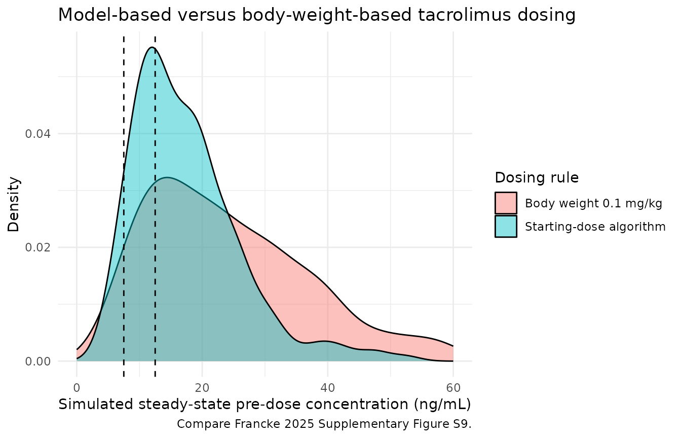
w_idx <- which(in_window$arm == "Body weight 0.1 mg/kg")
m_idx <- which(in_window$arm == "Starting-dose algorithm")
stopifnot(length(w_idx) == 1L, length(m_idx) == 1L)

# The paper's directional claim: model-based dosing narrows the spread of
# pre-dose concentrations relative to body-weight dosing.
stopifnot(in_window$`IQR width (ng/mL)`[m_idx] < in_window$`IQR width (ng/mL)`[w_idx])
The qualitative finding reproduces: the algorithm narrows the interquartile spread of pre-dose concentrations relative to body-weight dosing. The absolute percentages inside the 7.5-12.5 ng/mL window are shifted relative to the paper’s 28.4% and 33.2%, which follows directly from the AUC-to-trough discrepancy documented above – the algorithm is calibrated so that its concentrations centre on 10 ng/mL, and under the published structural model they centre near 16 ng/mL instead.
Assumptions and deviations
Extraction decisions
- Two model files, one vignette. Francke 2025 reports a base model, a final (full) model, and a starting-dose model. The base model is a model development step and is not distributed. The full model and the starting-dose model are both final, separately validated deliverables with complete parameter columns in Table 2 and separate prediction-corrected VPCs (Figures 2 and 4), so each is distributed as its own file.
-
IIV scale. Table 2’s
IIV (%)column is read as %CV, converted withomega^2 = log(1 + CV^2). See the scale check above: the %CV reading reproduces both the 19.3% and the 35% figures the paper quotes. -
Correlation matrix. Table 2 reports eta
correlations; the model files store covariances as
r_ij * omega_i * omega_j. Both resulting 3x3 blocks are positive definite. -
Residual error. Encoded as
lnorm()with the Table 2 values used directly as log-scale SDs, on the authority of the supplement’s$SIGMA 1 FIXconstruction. -
Missing covariates. The control stream maps every
missing covariate (
-999) to a multiplier of 1, i.e. to the centring value. The model files document this per covariate; a user supplying data must apply the same convention (substitute the centring value) rather than leavingNA. -
CYP3A5 “Other” genotype. The control stream assigns
the 1/3 multiplier to both
CYP3A5 == 2andCYP3A5 == 4, so the three recipients with an “Other” genotype are coded as heterozygotes. - Cohort marginals. The virtual cohort draws each continuous covariate independently from a log-normal matched to the Table 1 median and IQR. Francke 2025 does not report a covariate correlation structure, so correlations between age, height, weight, hematocrit, and creatinine are not reproduced. Genotype frequencies are renormalised over genotyped recipients.
- Figure 3 percentiles. The paper simulated the 10th, 25th, 50th, 75th, and 90th percentiles of each continuous covariate. Table 1 reports only the median and IQR, so the panels above use the 25th, 50th, and 75th percentiles.
-
Solver. The default
liblsodaintegrator fails on this model’sss = 1records; the vignette usesmethod = "lsoda"throughout.
Errata and inconsistencies in the source
-
Table 2 unit labels. The
K arow is headed(L/h); the parameter is a first-order absorption rate constant in 1/h, as the Abstract states (“the mean absorption rate was 6.59/h”). TheHeightrow is headed(m 2); the covariate is height in centimetres, as the supplement (CLHGT = ((HGT/170)**THETA(17))) and the Discussion (“height (in cm)”) both confirm, and as the centring constant 170 matching the Table 1 median height of 170 cm proves. - Explained variability quoted on two scales. The Abstract says the covariates “explained 19.3% of the inter-individual variability in clearance” while the Key Points, Results, and Conclusions say 35%. Both are correct: 19.3% is the reduction on the CV scale and 35% on the variance scale. This is not an error, but it is easy to misread.
-
The dosing algorithm mixes two models. The printed
starting-dose formula uses the covariate coefficients of the
starting-dose model (1.9, 0.842, -0.332, 0.97) but the typical CL/F of
the full model (20.7 L/h); the starting-dose model’s own CL/F
is 19.9 L/h. The formula is reproduced as printed, with
cl_constantexposed as an argument so a user can substitute 19.9 if the internally consistent version is wanted. - The 234 ng*h/mL AUC target is not consistent with the published structural model. The paper equates an AUC0-12h of 234 ng*h/mL with a 10 ng/mL pre-dose concentration (ratio 23.4). Simulating the published final model at any time after transplantation gives an AUC-to-trough ratio of about 14-15, so 234 ng*h/mL corresponds to a trough near 16.6 ng/mL and a 10 ng/mL trough corresponds to an AUC near 145-155 ng*h/mL. Section 3.4 says the constant was determined “on the basis of the data included in this study and the population pharmacokinetic model”, so the most likely explanation is that it was read off the observed AUC/trough pairs in the 208 densely sampled profiles rather than derived from the model. No parameter was adjusted to reconcile the two.
-
DATAversusCENTER. The supplement’s$ERRORblock switches the residual magnitude on a column calledDATA, but$INPUTlistsCENTERand noDATA. The published control stream does not reconcile the two names. The model files use a single canonical column,STUDY_TACRO_FRANCKE, holding the 1-7 stratum code the$ERRORblock expects. - Codes 1 vs 2 and 3 vs 4 are undocumented. The seven centre-by-method strata collapse onto five residual magnitudes; the paper never says what distinguishes stratum 1 from 2, or 3 from 4. Because each pair shares an estimated magnitude, the ambiguity has no effect on predictions.
Not implemented
- Inter-occasion variability. None is reported for either model.
- The time-after-transplantation effect (Equation 3) was evaluated by the authors and did not improve the model (Section 3.2.2), so it is not encoded.
-
The
V2COVhook. The control stream carriesV2COV = 1with no covariates on the central volume in the final model; nothing to encode. - Formulation effect on bioavailability. Prograf versus Adport was tested and estimated at exactly 1.0 after correcting for centre (Section 3.2.2), so formulation is not a covariate.
Session info
sessionInfo()
#> R version 4.6.1 (2026-06-24)
#> Platform: x86_64-pc-linux-gnu
#> Running under: Ubuntu 24.04.5 LTS
#>
#> Matrix products: default
#> BLAS:   /usr/lib/x86_64-linux-gnu/openblas-pthread/libblas.so.3
#> LAPACK: /usr/lib/x86_64-linux-gnu/openblas-pthread/libopenblasp-r0.3.26.so;  LAPACK version 3.12.0
#>
#> locale:
#>  [1] LC_CTYPE=C.UTF-8       LC_NUMERIC=C           LC_TIME=C.UTF-8
#>  [4] LC_COLLATE=C.UTF-8     LC_MONETARY=C.UTF-8    LC_MESSAGES=C.UTF-8
#>  [7] LC_PAPER=C.UTF-8       LC_NAME=C              LC_ADDRESS=C
#> [10] LC_TELEPHONE=C         LC_MEASUREMENT=C.UTF-8 LC_IDENTIFICATION=C
#>
#> time zone: UTC
#> tzcode source: system (glibc)
#>
#> attached base packages:
#> [1] stats     graphics  grDevices utils     datasets  methods   base
#>
#> other attached packages:
#> [1] ggplot2_4.0.3         dplyr_1.2.1           PKNCA_0.12.1
#> [4] rxode2_5.1.8          nlmixr2lib_0.3.2.9000
#>
#> loaded via a namespace (and not attached):
#>  [1] gtable_0.3.6        xfun_0.61           bslib_0.12.0
#>  [4] rxode2lincmt_0.1.0  lattice_0.22-9      vctrs_0.7.3
#>  [7] tools_4.6.1         generics_0.1.4      parallel_4.6.1
#> [10] tibble_3.3.1        symengine_0.2.14    pkgconfig_2.0.3
#> [13] data.table_1.18.6.1 checkmate_2.3.4     RColorBrewer_1.1-3
#> [16] S7_0.2.2            desc_1.4.3          lifecycle_1.0.5
#> [19] compiler_4.6.1      farver_2.1.2        textshaping_1.0.5
#> [22] fontawesome_0.5.3   htmltools_0.5.9     sys_3.4.3
#> [25] sass_0.4.10         yaml_2.3.12         tidyr_1.3.2
#> [28] pillar_1.11.1       pkgdown_2.2.1       crayon_1.5.3
#> [31] jquerylib_0.1.4     whisker_0.4.1       openssl_2.4.2
#> [34] cachem_1.1.0        nlme_3.1-169        tidyselect_1.2.1
#> [37] digest_0.6.39       lotri_1.0.5         purrr_1.2.2
#> [40] labeling_0.4.3      rxode2ll_2.0.18     fastmap_1.2.0
#> [43] grid_4.6.1          cli_3.6.6           dparser_1.3.1-14
#> [46] magrittr_2.0.5      withr_3.0.3         scales_1.4.0
#> [49] backports_1.5.1     rmarkdown_2.32      otel_0.2.0
#> [52] askpass_1.2.1       ragg_1.5.2          memoise_2.0.1
#> [55] evaluate_1.0.5      knitr_1.52          rex_1.2.2
#> [58] PreciseSums_0.7     rlang_1.3.0         downlit_0.4.5
#> [61] Rcpp_1.1.2          glue_1.8.1          xml2_1.6.0
#> [64] jsonlite_2.0.0      R6_2.6.1            systemfonts_1.3.2
#> [67] fs_2.1.0