Vancomycin in overweight and obese adults (Zhang 2024)
Source:vignettes/articles/Zhang_2024_vancomycin.Rmd
Zhang_2024_vancomycin.RmdModel and source
- Citation: Zhang T, Krekels EHJ, Smit C, van Dongen EPA, Bruggemann RJM, Knibbe CAJ. How to Dose Vancomycin in Overweight and Obese Patients with Varying Renal (Dys)function in the Novel Era of AUC 400-600 mg*h/L-Targeted Dosing. Clin Pharmacokinet. 2024;63(1):79-91. doi:10.1007/s40262-023-01324-5.
- Description: Three-compartment population PK model for intravenous vancomycin in overweight and obese hospitalised adults (ward and ICU) with varying renal function, pooled with morbidly obese otherwise healthy subjects undergoing bariatric surgery (Zhang 2024). Clearance scales with indexed CKD-EPI eGFR by a power function, linearly with total body weight, and is 15.5% lower in ICU patients. Residual error differs between the hospital-patient data (additive) and the AMIGO bariatric surgery data (combined), selected by STUDY_AMIGO.
- Article: https://doi.org/10.1007/s40262-023-01324-5 (open access, PMC10786964)
Zhang et al. pooled 1188 therapeutic-drug-monitoring (TDM) vancomycin
concentrations from 210 overweight and obese hospitalised patients with
varying renal function (ward and ICU) with 207 rich-sampling
concentrations from 20 morbidly obese, otherwise healthy subjects given
a single dose during bariatric surgery (the AMIGO trial, published as
Smit 2020 and available here as Smit_2020_vancomycin). A
three-compartment model was fitted in NONMEM 7.4 (FOCE-I). Clearance
increases with indexed CKD-EPI eGFR (power exponent 0.658) and linearly
with total body weight, and is 15.5% lower in ICU patients. The authors
used the model to derive AUC24 400-600 mg*h/L-targeted dosing tables for
continuous and intermittent infusion (Figures 2-5) and showed the
resulting daily AUC24 over the first week (Figures 6 and 7).
Population
The 230 subjects (Table 1) were 140 men and 90 women, median age 70 years (23-92), median total body weight 91.8 kg (58.6-234.6) and median BMI 30.0 kg/m^2 (25.0-65.7). The 210 TDM patients (157 ward, 53 ICU) were overweight or obese (BMI >= 25 kg/m^2) with indexed CKD-EPI from 6.0 to 154.9 mL/min/1.73 m^2 (median 73.7); patients on renal replacement therapy were excluded. The 20 AMIGO subjects (BMI 40.8-65.7 kg/m^2, median weight 141.2 kg) all had eGFR >= 60 mL/min/1.73 m^2 and received 12.5 mg/kg (maximum 2500 mg) as a single infusion. All subjects were treated at St. Antonius Hospital, Nieuwegein, the Netherlands.
The same information is available programmatically via
readModelDb("Zhang_2024_vancomycin")()$population.
Source trace
The per-parameter origin is recorded as an in-file comment next to
each ini() entry in
inst/modeldb/specificDrugs/Zhang_2024_vancomycin.R. The
table below collects them in one place.
| Equation / parameter | Value | Source location |
|---|---|---|
lcl (TVCL) |
log(3.36 L/h) | Table 2, TVCL (RSE 2.60%) |
lvc (V1) |
log(16.7 L) | Table 2, V1 (RSE 14.0%) |
lq (Q2) |
log(16.1 L/h) | Table 2, Q2 (RSE 11.5%) |
lvp (V2) |
log(23.1 L) | Table 2, V2 (RSE 3.60%) |
lq2 (Q3) |
log(2.44 L/h) | Table 2, Q3 (RSE 8.00%) |
lvp2 (V3) |
log(83.0 L) | Table 2, V3 (RSE 4.50%) |
e_crcl_cl (theta1) |
0.658 | Table 2, theta1 (RSE 3.10%) |
e_wt_cl (theta2) |
0.0106 1/kg | Table 2, theta2 (RSE 13.8%) |
e_dis_critill_cl (FICU) |
0.845 | Table 2, FICU (RSE 2.30%); footnote a: 1 if not in ICU |
etalcl |
0.0730 (variance) | Table 2, IIV CL |
etalvc |
0.978 (variance) | Table 2, IIV V1 |
addSd |
sqrt(9.32) = 3.0529 mg/L | Table 2, PA data additive error (variance) |
propSd_amigo |
sqrt(0.00216) = 0.046476 | Table 2, HS data proportional error (variance) |
addSd_amigo |
sqrt(1.10) = 1.0488 mg/L | Table 2, HS data additive error (variance) |
| CL equation | TVCL * (CKDEPI/75)^theta1 * [1 + theta2 * (TBW - 90)] * FICU |
Table 2, first row |
| Three-compartment structure, IIV on CL and V1 only | n/a | Results, Population Pharmacokinetic Analysis |
Typical-value clearance
The paper states that “CL was 3.36 L/h in a typical patient … For a patient admitted to the ICU, this value was 2.84 L/h”. The model reproduces both values at the centring values of the Table 2 equation.
cl_typ <- function(CRCL, WT, ICU) {
  3.36 * (CRCL / 75)^0.658 * (1 + 0.0106 * (WT - 90)) * 0.845^ICU
}
mod <- readModelDb("Zhang_2024_vancomycin")
ref_ev <- data.frame(
  id = 1:2, time = 0, evid = 0, amt = 0, cmt = "central",
  CRCL = 75, WT = 90, DIS_CRITILL = c(0, 1), STUDY_AMIGO = 0
)
ref_cl <- rxode2::rxSolve(rxode2::zeroRe(mod), events = ref_ev)$cl
ref_cl
#> [1] 3.3600 2.8392
stopifnot(
  abs(ref_cl[1] - 3.36) < 1e-6,
  abs(round(ref_cl[2], 2) - 2.84) < 1e-9,
  abs(ref_cl[2] - cl_typ(75, 90, 1)) < 1e-6
)
Virtual cohort
Figures 6 and 7 of the paper simulate representative virtual patients with indexed CKD-EPI of 100, 80, 60, 40 and 20 mL/min/1.73 m^2 and total body weight of 80, 120, 160 and 200 kg, each dosed according to the paper’s dosing tables: Figure 2 (ward, continuous infusion), Figure 3 (ward, intermittent), Figure 4 (ICU, continuous infusion) and Figure 5 (ICU, intermittent). The tables below were transcribed by the maintainers from those figures. The paper ran 1000 simulations per patient type; 100 are used here (2000 subjects per regimen).
wt_levels <- c(80, 120, 160, 200)
crcl_levels <- c(100, 80, 60, 40, 20)
wt_band_lab <- c("TBW 70-100", "TBW 100-140", "TBW 140-180", "TBW >180")
crcl_band_lab <- c("CKD >90", "CKD 70-90", "CKD 50-70", "CKD 30-50", "CKD 10-30")

# Rows: TBW 70-100, 100-140, 140-180, >180.
# Columns: CKD-EPI >90, 70-90, 50-70, 30-50, 10-30 (mL/min/1.73 m^2).
dose_tab <- function(x) matrix(x, nrow = 4, byrow = TRUE)
tables <- list(
  # Continuous infusion maintenance, mg/24 h (Figures 2 and 4).
  ward_ci = dose_tab(c(
    2000, 1750, 1500, 1250, 750,
    2750, 2500, 2000, 1500, 1000,
    3750, 3250, 2750, 2000, 1250,
    4500, 4000, 3250, 2500, 1750
  )),
  icu_ci = dose_tab(c(
    1750, 1500, 1250, 1000, 750,
    2250, 2000, 1750, 1250, 1000,
    3000, 2750, 2250, 1750, 1250,
    3750, 3500, 2750, 2000, 1500
  )),
  # Intermittent: two loading doses at 0 and 12 h (mg per 2-h infusion).
  ward_ld = dose_tab(c(
    1750, 1500, 1500, 1250, 1250,
    2250, 2000, 1750, 1500, 1250,
    2500, 2250, 2250, 1750, 1500,
    3000, 2750, 2500, 2000, 1500
  )),
  icu_ld = dose_tab(c(
    2000, 1500, 1500, 1250, 1250,
    2250, 1750, 1500, 1500, 1250,
    2250, 2000, 2000, 1750, 1500,
    2750, 2250, 2250, 2000, 1500
  )),
  # Intermittent maintenance from day 2 (mg per 2-h infusion) and interval (h).
  ward_md = dose_tab(c(
    1000, 1000, 1500, 1000, 750,
    1500, 1250, 2000, 1500, 1000,
    1750, 1500, 1250, 1000, 1250,
    2250, 2000, 1750, 1250, 1750
  )),
  ward_tau = dose_tab(c(
    12, 12, 24, 24, 24,
    12, 12, 24, 24, 24,
    12, 12, 12, 12, 24,
    12, 12, 12, 12, 24
  )),
  icu_md = dose_tab(c(
    750, 750, 1250, 1000, 750,
    1000, 1000, 1750, 1250, 1000,
    1500, 1250, 1250, 1000, 1000,
    2000, 1750, 1500, 1000, 1250
  )),
  icu_tau = dose_tab(c(
    12, 12, 24, 24, 24,
    12, 12, 24, 24, 24,
    12, 12, 12, 12, 24,
    12, 12, 12, 12, 24
  ))
)
The continuous-infusion schedule (Figures 2 and 4) is a 1500 mg loading infusion over 0-2 h, the maintenance infusion from 2 to 26 h, a second 750 mg loading infusion over 26-28 h, and the maintenance infusion again from 28 h onwards. The intermittent schedule (Figures 3 and 5) is two loading doses as 2-h infusions at 0 and 12 h, then maintenance 2-h infusions every 12 or 24 h from 24 h.
n_per_cell <- 100L
t_end <- 168
obs_times <- seq(0, t_end, by = 1)

cell_doses <- function(setting, regimen, i, j) {
  if (regimen == "Continuous infusion") {
    md <- tables[[paste0(setting, "_ci")]][i, j]
    rate <- md / 24
    data.frame(
      time = c(0, 2, 26, 28),
      amt = c(1500, md, 750, rate * (t_end - 28)),
      rate = c(750, rate, 375, rate)
    )
  } else {
    ld <- tables[[paste0(setting, "_ld")]][i, j]
    md <- tables[[paste0(setting, "_md")]][i, j]
    tau <- tables[[paste0(setting, "_tau")]][i, j]
    md_times <- seq(24, t_end - 1, by = tau)
    data.frame(
      time = c(0, 12, md_times),
      amt = c(ld, ld, rep(md, length(md_times))),
      rate = c(ld, ld, rep(md, length(md_times))) / 2
    )
  }
}

make_cell <- function(setting, regimen, i, j, id_offset) {
  ids <- id_offset + seq_len(n_per_cell)
  doses <- cell_doses(setting, regimen, i, j)
  dose_rows <- tidyr::expand_grid(id = ids, doses) |>
    mutate(evid = 1L)
  obs_rows <- tidyr::expand_grid(id = ids, time = obs_times) |>
    mutate(evid = 0L, amt = 0, rate = 0)
  bind_rows(dose_rows, obs_rows) |>
    mutate(
      cmt = "central",
      WT = wt_levels[i],
      CRCL = crcl_levels[j],
      DIS_CRITILL = as.integer(setting == "icu"),
      STUDY_AMIGO = 0L,
      setting = if (setting == "icu") "ICU" else "Ward",
      regimen = regimen,
      wt_band = wt_band_lab[i],
      crcl_band = crcl_band_lab[j]
    )
}

scenarios <- tidyr::expand_grid(
  setting = c("ward", "icu"),
  regimen = c("Continuous infusion", "Intermittent"),
  i = seq_along(wt_levels),
  j = seq_along(crcl_levels)
)
events <- bind_rows(lapply(seq_len(nrow(scenarios)), function(k) {
  s <- scenarios[k, ]
  make_cell(s$setting, s$regimen, s$i, s$j, id_offset = (k - 1L) * n_per_cell)
})) |>
  arrange(id, time, desc(evid))
stopifnot(!anyDuplicated(unique(events[, c("id", "time", "evid", "amt")])))
length(unique(events$id))
#> [1] 8000
Simulation
rxode2::rxSetSeed(20240101)
sim <- rxode2::rxSolve(
  mod,
  events = events,
  keep = c("setting", "regimen", "wt_band", "crcl_band")
) |>
  as.data.frame()
#> ℹ parameter labels from comments will be replaced by 'label()'
Daily AUC24 is the linear-trapezoidal area of the individual
concentration Cc over each 24-h day, from the hourly
grid.
daily_auc <- sim |>
  arrange(id, time) |>
  group_by(id) |>
  mutate(seg = (Cc + lag(Cc)) / 2 * (time - lag(time)), day = ceiling(time / 24)) |>
  filter(time > 0) |>
  group_by(id, setting, regimen, wt_band, crcl_band, day) |>
  summarise(auc24 = sum(seg), .groups = "drop") |>
  mutate(
    wt_band = factor(wt_band, levels = wt_band_lab),
    crcl_band = factor(crcl_band, levels = crcl_band_lab)
  )

auc_summary <- daily_auc |>
  group_by(setting, regimen, wt_band, crcl_band, day) |>
  summarise(
    Q025 = quantile(auc24, 0.025),
    Q50 = median(auc24),
    Q975 = quantile(auc24, 0.975),
    .groups = "drop"
  )
Replicate published figures
plot_auc <- function(which_setting, fig) {
  auc_summary |>
    filter(setting == which_setting) |>
    ggplot(aes(day, Q50)) +
    geom_ribbon(aes(ymin = Q025, ymax = Q975), fill = "grey80") +
    geom_line() +
    geom_hline(yintercept = c(400, 600), linetype = "dashed") +
    facet_grid(crcl_band ~ regimen + wt_band) +
    scale_x_continuous(breaks = 1:7) +
    labs(
      x = "Time (days)", y = "AUC24 (mg*h/L)",
      title = paste0("Figure ", fig, " (a, b): daily AUC24, ", which_setting, " patients"),
      caption = paste0("Replicates Figure ", fig, "a,b of Zhang 2024. Median and 95% prediction interval.")
    ) +
    theme(strip.text = element_text(size = 7), axis.text.x = element_text(size = 6))
}
plot_auc("Ward", 6)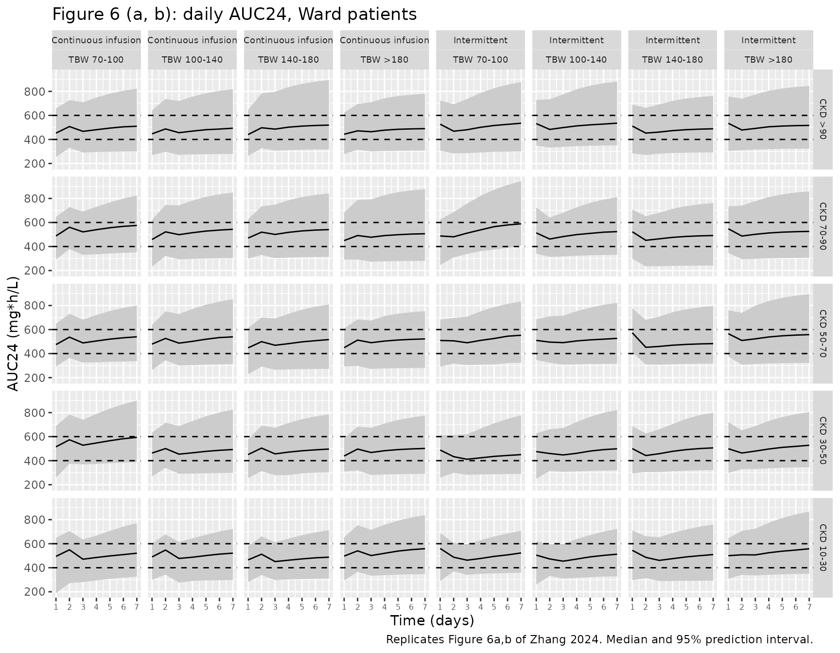
plot_auc("ICU", 7)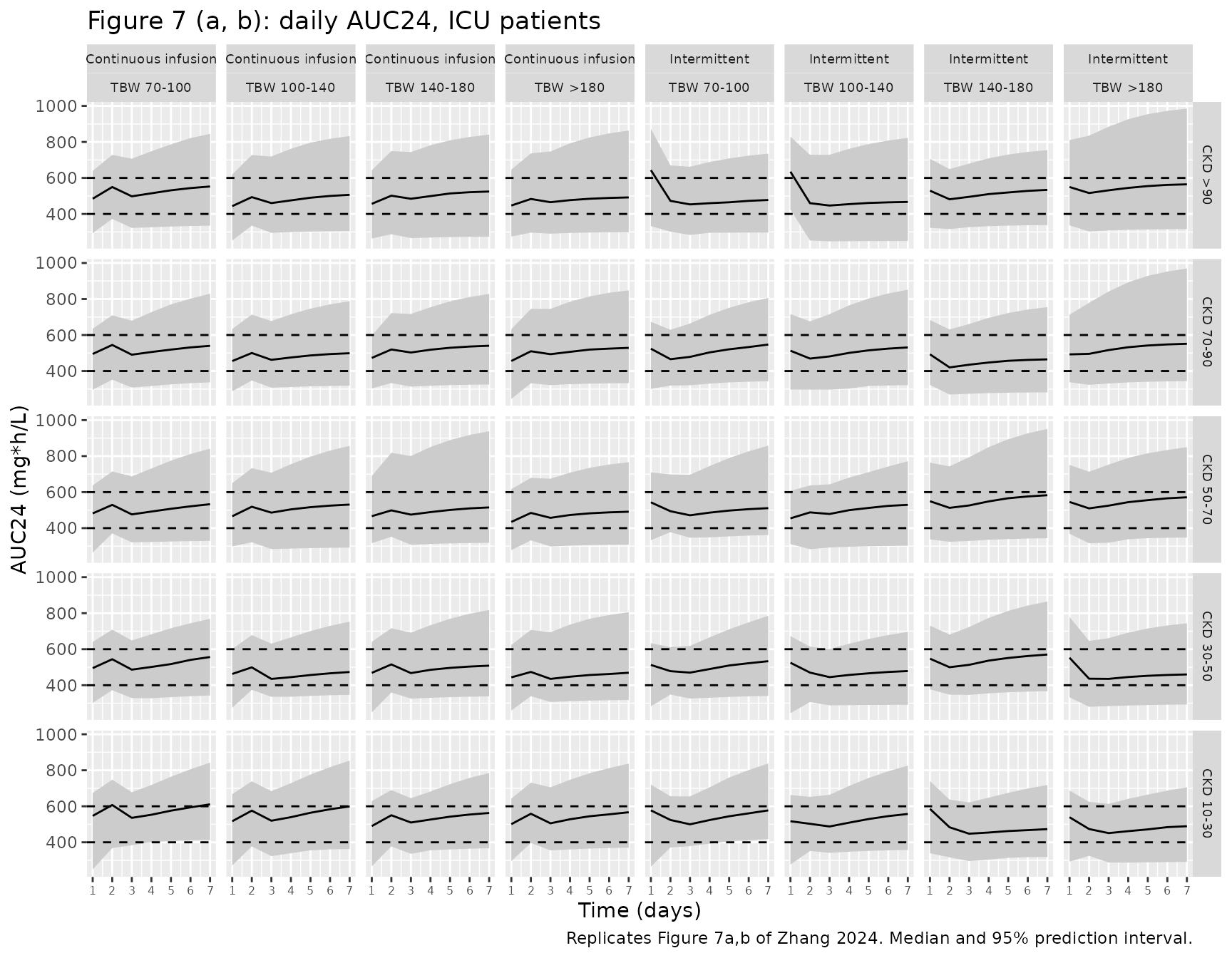
plot_conc <- function(which_setting, fig) {
  sim |>
    filter(setting == which_setting) |>
    mutate(
      wt_band = factor(wt_band, levels = wt_band_lab),
      crcl_band = factor(crcl_band, levels = crcl_band_lab)
    ) |>
    group_by(regimen, wt_band, crcl_band, time) |>
    summarise(
      Q025 = quantile(Cc, 0.025), Q50 = median(Cc), Q975 = quantile(Cc, 0.975),
      .groups = "drop"
    ) |>
    ggplot(aes(time / 24, Q50)) +
    geom_ribbon(aes(ymin = Q025, ymax = Q975), fill = "grey80") +
    geom_line() +
    facet_grid(crcl_band ~ regimen + wt_band) +
    scale_x_continuous(breaks = 0:7) +
    labs(
      x = "Time (days)", y = "Vancomycin concentration (mg/L)",
      title = paste0("Figure ", fig, " (c, d): concentrations, ", which_setting, " patients"),
      caption = paste0("Replicates Figure ", fig, "c,d of Zhang 2024.")
    ) +
    theme(strip.text = element_text(size = 7), axis.text.x = element_text(size = 6))
}
plot_conc("Ward", 6)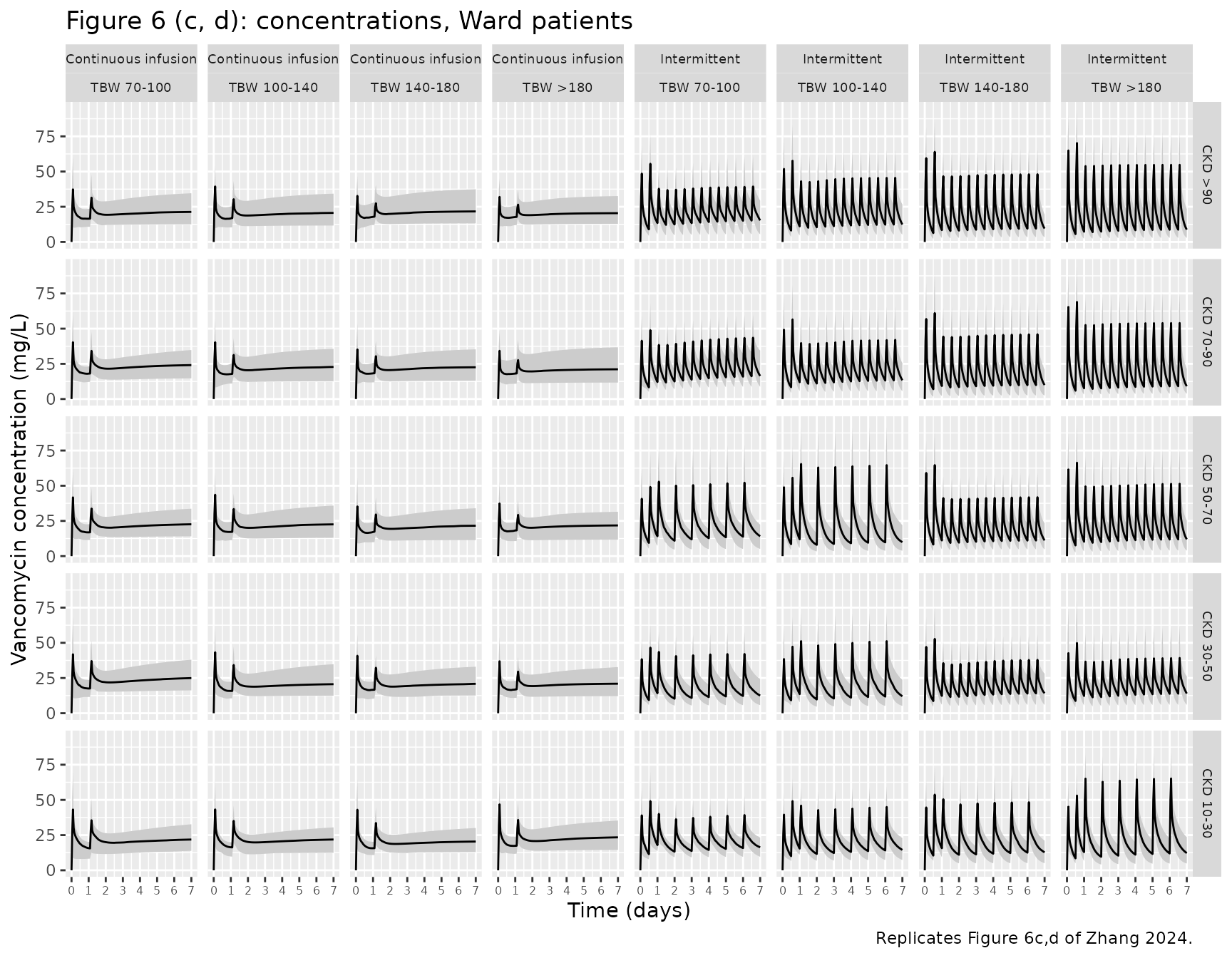
plot_conc("ICU", 7)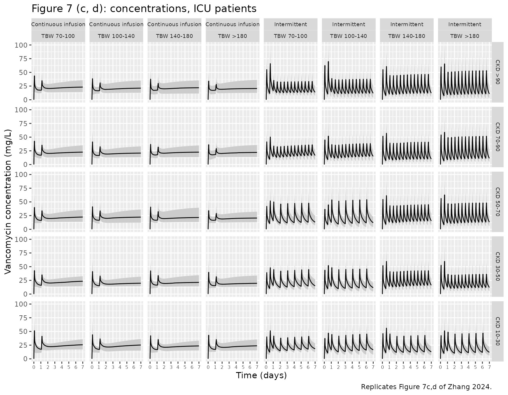
The paper states that with the proposed dosing tables “the median AUC24 is within the target of 400-600 mgh/L, regardless of renal function, bodyweight, and ICU admission status, even though for some ICU subgroups AUC may be slightly above 600 mgh/L”. The check below asserts this on the centre of the simulated distribution: the median over the 80 regimen x setting x weight x renal-function cells of the per-cell day-7 median AUC24 lies within the target, and every per-cell day-7 median lies within a wide envelope around it (a mis-transcribed clearance, exponent or centring value moves whole cells by tens of percent).
day7 <- auc_summary |> filter(day == 7)
day1 <- auc_summary |> filter(day == 1)
summary(day7$Q50)
#>    Min. 1st Qu.  Median    Mean 3rd Qu.    Max.
#>   450.4   498.2   524.2   524.4   548.2   610.9
summary(day1$Q50)
#>    Min. 1st Qu.  Median    Mean 3rd Qu.    Max.
#>   434.4   464.7   494.8   500.4   527.5   643.3
stopifnot(
  median(day7$Q50) > 400, median(day7$Q50) < 600,
  all(day7$Q50 > 350), all(day7$Q50 < 750),
  median(day1$Q50) > 400, median(day1$Q50) < 600
)
PKNCA validation
The paper reports the concentrations reached with its dosing tables “across the entire patient population”: median (interquartile range) 23.08 (19.54-27.29) mg/L for continuous infusion and a trough of 16.89 (12.65-20.50) mg/L for intermittent dosing. PKNCA computes the day-7 (144-168 h) average concentration and minimum concentration per simulated subject, together with the day-1 and day-7 AUC. To keep the render fast, PKNCA uses the first 20 simulated subjects of every patient type (1600 subjects) and only the concentrations inside the two intervals.
nca_ids <- unique(events$id[(events$id - 1L) %% n_per_cell < 20L])
sim_nca <- sim |>
  filter(!is.na(Cc), id %in% nca_ids, time <= 24 | time >= 144) |>
  select(id, time, Cc, setting, regimen)
sim_nca <- bind_rows(
  sim_nca,
  sim_nca |> distinct(id, setting, regimen) |> mutate(time = 0, Cc = 0)
) |>
  distinct(id, setting, regimen, time, .keep_all = TRUE) |>
  arrange(id, time)

dose_df <- events |>
  filter(evid == 1, id %in% nca_ids) |>
  select(id, time, amt, setting, regimen)

conc_obj <- PKNCA::PKNCAconc(sim_nca, Cc ~ time | regimen + setting + id)
dose_obj <- PKNCA::PKNCAdose(dose_df, amt ~ time | regimen + setting + id)
intervals <- data.frame(
  start = c(0, 144),
  end = c(24, 168),
  auclast = TRUE,
  cav = c(FALSE, TRUE),
  cmin = c(FALSE, TRUE)
)
nca_res <- PKNCA::pk.nca(PKNCA::PKNCAdata(
  conc_obj, dose_obj,
  intervals = intervals, options = list(auc.method = "linear", progress = FALSE)
))
nca_df <- as.data.frame(nca_res)
PKNCA’s linear-trapezoidal AUC and the hand-computed daily AUC above use the same data and the same rule, so they agree to numerical precision.
pk_auc <- nca_df |>
  filter(PPTESTCD == "auclast") |>
  mutate(day = end / 24) |>
  select(id, day, PPORRES)
both <- inner_join(pk_auc, daily_auc |> select(id, day, auc24), by = c("id", "day"))
stopifnot(nrow(both) == 2 * length(nca_ids), max(abs(both$PPORRES - both$auc24)) < 1e-6)
nca_day7 <- nca_df |> filter(start == 144)
sim_ci <- nca_day7 |>
  filter(regimen == "Continuous infusion", PPTESTCD == "cav")
sim_ii <- nca_day7 |>
  filter(regimen == "Intermittent", PPTESTCD == "cmin")
simulated <- bind_rows(sim_ci, sim_ii) |>
  select(regimen, PPTESTCD, PPORRES)
published <- tibble::tribble(
  ~regimen, ~cav, ~cmin,
  "Continuous infusion", 23.08, NA,
  "Intermittent", NA, 16.89
)
cmp <- nlmixr2lib::ncaComparisonTable(
  simulated = simulated,
  reference = published,
  by = "regimen",
  units = c(cav = "mg/L", cmin = "mg/L"),
  tolerance_pct = 20
)
knitr::kable(
  cmp,
  caption = paste(
    "Day-7 simulated concentration (median over ward and ICU subjects of all",
    "weight and renal-function cells) vs. the medians reported in the Results",
    "of Zhang 2024. * differs from reference by >20%."
  )
)| NCA parameter | regimen | Reference | Simulated | % diff |
|---|---|---|---|---|
| Cmin (mg/L) | Intermittent | 16.9 | 13.1 | -22.3%* |
| Cavg (mg/L) | Continuous infusion | 23.1 | 21.7 | -6.1% |
iqr_tab <- bind_rows(sim_ci, sim_ii) |>
  group_by(regimen, PPTESTCD) |>
  summarise(
    median = median(PPORRES),
    q25 = quantile(PPORRES, 0.25),
    q75 = quantile(PPORRES, 0.75),
    .groups = "drop"
  ) |>
  mutate(published = c("23.08 (19.54-27.29)", "16.89 (12.65-20.50)"))
iqr_tab |>
  rename(
    "Regimen" = regimen, "Parameter" = PPTESTCD, "Simulated median" = median,
    "Simulated Q25" = q25, "Simulated Q75" = q75, "Published median (IQR)" = published
  ) |>
knitr::kable(digits = 2)| Regimen | Parameter | Simulated median | Simulated Q25 | Simulated Q75 | Published median (IQR) |
|---|---|---|---|---|---|
| Continuous infusion | cav | 21.68 | 18.30 | 26.00 | 23.08 (19.54-27.29) |
| Intermittent | cmin | 13.13 | 8.98 | 17.27 | 16.89 (12.65-20.50) |
# Continuous infusion: the average concentration is AUC24 / 24, so a
# mis-transcribed clearance or dosing table moves it by tens of percent.
# The intermittent trough is a known deviation (see below) and is not gated.
stopifnot(abs(iqr_tab$median[1] / 23.08 - 1) < 0.15)
The continuous-infusion average concentration matches the published median. The simulated day-7 intermittent trough (median about 13 mg/L) is about 22% below the published 16.89 mg/L. The paper’s own concentration figures agree with the simulation rather than with that number: in Figures 6d and 7d of the paper the median intermittent troughs fall below the 15 mg/L dashed line in many panels, and the daily AUC24 of the same regimens (Figures 6b and 7b) is reproduced above. The paper does not say how its pooled trough was defined (which doses, which days, which patient types), so the difference is recorded here as a known deviation rather than a model error.
The paper does not say which day, or which ward/ICU mix, its pooled concentrations summarise; the comparison here uses day 7 and weights the ward and ICU cells equally.
Assumptions and deviations
-
Centring weight of the TBW effect. The Table 2
equation centres total body weight at 90 kg,
[1 + theta2 * (TBW - 90)], while the Results text describes TVCL = 3.36 L/h as the clearance of “a typical patient with a TBW of 100 kg”. The model follows the equation. The paper’s own dosing simulations support it: with the Figure 2 continuous-infusion doses, the steady-state AUC24 (dose / CL) of the representative ward patients is 510-629 mgh/L under 90 kg centring, matching Figure 6a, but 538-714 mgh/L under 100 kg centring, which would put the 80-kg patients above the 600 mg*h/L safety limit that Figure 6a shows them within. - Residual-error units. Table 2 labels the additive residual errors “L/mg” and reports them as variances. They are read as variances in (mg/L)^2 and converted to standard deviations: 3.05 mg/L (patients) and 1.05 mg/L (AMIGO).
-
Dataset-specific residual error. Table 2 reports an
additive error for the hospital-patient (‘PA’) data and a combined
additive + proportional error for the bariatric-surgery (‘HS’) data. The
new indicator
STUDY_AMIGO(1 = AMIGO record) selects between them. It has no effect on any structural or IIV parameter. Simulations of patients should setSTUDY_AMIGO = 0. -
ICU indicator. ICU admission status (FICU) is
encoded with the canonical
DIS_CRITILL(1 = ICU), as0.845^DIS_CRITILLon clearance. - Time-varying renal function. CKD-EPI was time-varying in the analysis (median 11 serum creatinine measurements per patient). It is held constant per virtual patient here, as in the paper’s dosing simulations.
- Simulation size and loading-dose timing. 100 simulated subjects per patient type (the paper used 1000). The continuous-infusion maintenance infusion is paused during the 2-h day-2 loading infusion (26-28 h), which is how the timelines in Figures 2 and 4 draw it. The dosing tables were transcribed by the maintainers from Figures 2-5.
- No errata. No correction notice for this article was found as of 2026-10-28.