Ponezumab (Nicholas 2009)
Source:vignettes/articles/Nicholas_2009_ponezumab.Rmd
Nicholas_2009_ponezumab.RmdModel and source
- Citation: Nicholas T, Knebel W, Gastonguay MR, Bednar MM, Billing B, Landen JW, Kupiec JW, Corrigan B, Laurencot R, Zhao Q. Preliminary population pharmacokinetic modeling of PF-04360365, a humanized anti-amyloid monoclonal antibody, in patients with mild-to-moderate alzheimer’s disease. Alzheimers Dement. 2009;5(4 Suppl):P425. doi:10.1016/j.jalz.2009.04.270
- Description: Two-compartment intravenous population PK model for PF-04360365 (ponezumab), a humanized anti-amyloid IgG2 delta-a monoclonal antibody, in adults with mild-to-moderate Alzheimer’s disease; allometric body-weight scaling with estimated exponents on every disposition parameter and a full 4x4 inter-individual block on (CL, V1, V2, Q) (Nicholas 2009 preliminary popPK)
- Article: doi:10.1016/j.jalz.2009.04.270
- Open-access conference poster (Metrum/Pfizer): https://metrumrg.com/wp-content/uploads/2018/08/PK_modeling_in_mild_-_mod.pdf
Nicholas 2009 is a conference poster presented at the Alzheimer’s Association International Conference 2009 and indexed in the Alzheimer’s and Dementia supplement. It describes a preliminary two-compartment intravenous population PK model for PF-04360365 (later named ponezumab), a humanized anti-amyloid IgG2 delta-a monoclonal antibody developed by Pfizer (Rinat) and discontinued after Phase II.
Population
Nicholas 2009 fit the model to plasma PK data from 26 patients with mild-to-moderate Alzheimer’s disease (Mini Mental State Examination score 16-26) in a randomized, double-blind, placebo-controlled, dose-escalation study (a further 11 placebo subjects were not used in the analysis). Single intravenous doses of PF-04360365 spanning 0.1 to 10 mg/kg were administered. Patients were aged 60 to 80 years; weight and sex distributions are not tabulated in the poster.
Plasma drug concentrations were measured by ELISA over an analytical range of 156 to 10,000 ng/mL with intra- and inter-assay precisions within 10 percent and accuracy (percent relative error) at or below 16.0 percent. Concentrations below the lower limit of quantification or otherwise missing were excluded from the analysis, and subjects with no quantifiable concentrations were dropped from the fit. The poster states that covariate analysis was limited to the effect of body weight (allometric scaling on every disposition parameter, with reference 70 kg) because the small sample size and narrow age range did not support broader covariate exploration.
The same information is available programmatically via
readModelDb("Nicholas_2009_ponezumab")$population.
Source trace
The per-parameter origin is recorded as an in-file comment next to
each ini() entry in
inst/modeldb/specificDrugs/Nicholas_2009_ponezumab.R. The
table below collects them in one place for review.
| Equation / parameter | Value | Source location |
|---|---|---|
lcl (CL at WT=70 kg) |
0.00684 L/h | Nicholas 2009 Table 1 Theta_1 (6% SE; 95% CI 0.00597-0.00771) |
lvc (V1 at WT=70 kg) |
3.16 L | Nicholas 2009 Table 1 Theta_2 (3% SE; 95% CI 2.95-3.37) |
lq (Q at WT=70 kg) |
0.0210 L/h | Nicholas 2009 Table 1 Theta_3 (10% SE; 95% CI 0.0170-0.0250) |
lvp (V2 at WT=70 kg) |
5.34 L | Nicholas 2009 Table 1 Theta_4 (8% SE; 95% CI 4.49-6.18) |
e_wt_cl (WT exp on CL) |
0.911 | Nicholas 2009 Table 1 Theta_5 (37% SE; 95% CI 0.370-1.45) |
e_wt_vc (WT exp on V1) |
0.573 | Nicholas 2009 Table 1 Theta_6 (34% SE; 95% CI 0.194-0.951) |
e_wt_q (WT exp on Q) |
0.236 | Nicholas 2009 Table 1 Theta_7 (126% SE; 95% CI -0.346-0.817) |
e_wt_vp (WT exp on V2) |
0.590 | Nicholas 2009 Table 1 Theta_8 (54% SE; 95% CI -0.0288-1.20) |
| OMEGA 4x4 block on (CL, V1, V2, Q) | see file | Nicholas 2009 Table 1 inter-individual variance; full block omega per Methods |
propSd (proportional SD) |
0.0999 | Nicholas 2009 Table 1 sigma^2 prop = 0.00998 (11% SE); SD = sqrt(0.00998) |
d/dt(central) <- -kel*central - k12*central + k21*peripheral1 |
n/a | Nicholas 2009 Methods: “two-compartment model … implemented using ADVAN 3 TRANS4” |
d/dt(peripheral1) <- k12*central - k21*peripheral1 |
n/a | Nicholas 2009 Methods: ADVAN3 TRANS4 |
| Reference weight 70 kg for the allometric power scaling | 70 kg | Nicholas 2009 Methods: “Allometric scaling was implemented using a reference weight of 70 kg.” |
| Exponential IIV (log-normal) on disposition parameters | n/a | Nicholas 2009 Methods: “Inter-individual random effects were modeled with exponential variance models. Covariance was described with a full block omega matrix.” |
| Proportional residual error structure | n/a | Nicholas 2009 Methods: “a proportional error model was utilized for the residual error model.” |
Virtual cohort
The original observed data are not publicly available. The figures below use a virtual population whose dose distribution spans the published 0.1-10 mg/kg range and whose body-weight distribution approximates a typical mild-to-moderate Alzheimer’s disease cohort (median 70 kg, range about 50-100 kg). The published study enrolled 26 active subjects across the dose-escalation cohorts; we use 25 subjects per dose level (well below the 200-per-arm validation cap) to characterise the typical-value response and the inter-individual spread at each dose.
set.seed(20260625L)

dose_levels_mgkg <- c(0.1, 0.3, 1, 3, 10)
n_per_dose       <- 25L

make_cohort <- function(n, dose_mgkg, id_offset) {
  weights <- pmax(pmin(stats::rnorm(n, mean = 70, sd = 12), 100), 50)
  tibble::tibble(
    id      = id_offset + seq_len(n),
    WT      = weights,
    dose_mgkg = dose_mgkg,
    amt_mg    = dose_mgkg * weights
  )
}

subjects <- dplyr::bind_rows(
  lapply(seq_along(dose_levels_mgkg), function(i) {
    make_cohort(
      n         = n_per_dose,
      dose_mgkg = dose_levels_mgkg[i],
      id_offset = (i - 1L) * n_per_dose
    )
  })
)

# Dose row: single IV bolus into central at time 0.
dose_rows <- subjects |>
  dplyr::mutate(
    time = 0,
    evid = 1L,
    amt  = amt_mg,
    cmt  = "central",
    treatment = paste0(dose_mgkg, " mg/kg")
  ) |>
  dplyr::select(id, time, evid, amt, cmt, WT, dose_mgkg, treatment)

# Observation grid: dense early for Cmax/distribution, then weekly to ~day 85
# and biweekly out to ~day 168 to characterise the terminal phase.
obs_times_h <- c(
  seq(0, 24, by = 2),
  seq(48, 24 * 7, by = 12),
  seq(24 * 8, 24 * 85, by = 24),
  seq(24 * 91, 24 * 168, by = 24 * 7)
)

obs_rows <- tidyr::expand_grid(
  subjects |> dplyr::select(id, WT, dose_mgkg) |>
    dplyr::mutate(treatment = paste0(dose_mgkg, " mg/kg")),
  time = obs_times_h
) |>
  dplyr::mutate(
    evid = 0L,
    amt  = NA_real_,
    cmt  = "central"
  ) |>
  dplyr::select(id, time, evid, amt, cmt, WT, dose_mgkg, treatment)

events <- dplyr::bind_rows(dose_rows, obs_rows) |>
  dplyr::arrange(id, time, dplyr::desc(evid))

stopifnot(!anyDuplicated(unique(events[, c("id", "time", "evid")])))
Simulation
mod <- readModelDb("Nicholas_2009_ponezumab")
sim <- rxode2::rxSolve(mod, events = events, keep = c("WT", "dose_mgkg", "treatment")) |>
  as.data.frame()
#> ℹ parameter labels from comments will be replaced by 'label()'
For deterministic replication (no between-subject variability), zero out the random effects:
mod_typical <- mod |> rxode2::zeroRe()
#> ℹ parameter labels from comments will be replaced by 'label()'
sim_typical <- rxode2::rxSolve(mod_typical, events = events,
                               keep = c("WT", "dose_mgkg", "treatment")) |>
  as.data.frame()
#> ℹ omega/sigma items treated as zero: 'etalcl', 'etalvc', 'etalvp', 'etalq'
#> Warning: multi-subject simulation without without 'omega'
Replicate published figures
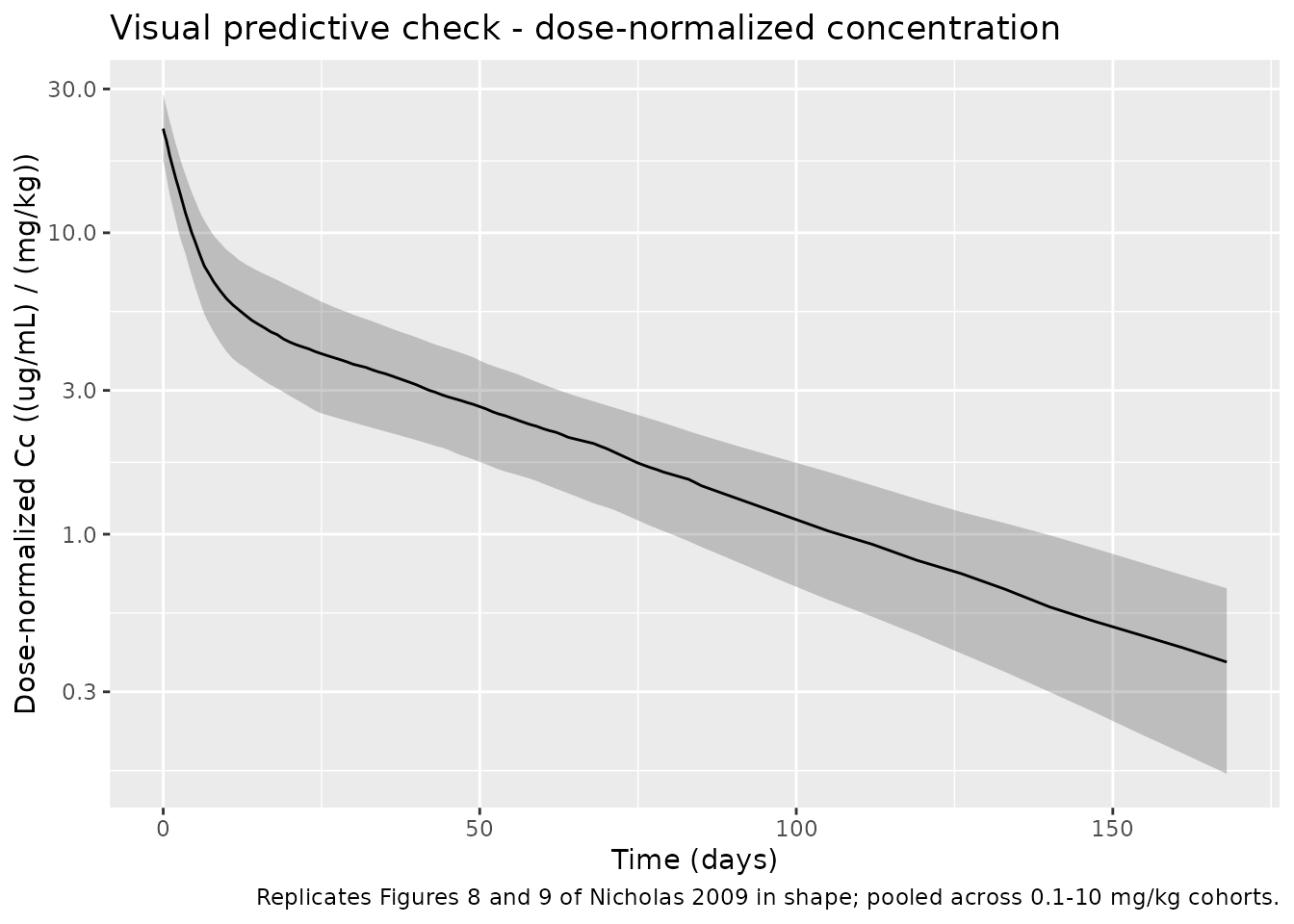
Figure 8/9 - Visual predictive check (dose-normalized concentration)
Nicholas 2009 Figures 8 and 9 present visual predictive checks for plasma PF-04360365 concentrations with 80% prediction intervals. Figure 8 covers day 1 to 85, and Figure 9 covers all post-dose data. Both plot dose-normalised concentrations on a log scale. The replication here is the 80% prediction interval (5th and 95th percentiles) of the simulated dose-normalised concentration over time, pooled across the 0.1-10 mg/kg range. The poster does not provide per-time-point reference values, so this replication is qualitative (shape of the median + bounds) rather than a point comparison.
vpc_dn <- sim |>
  dplyr::filter(!is.na(Cc)) |>
  dplyr::mutate(time_day = time / 24,
                Cc_dn    = ifelse(Cc > 0, Cc / dose_mgkg, NA_real_)) |>
  dplyr::group_by(time_day) |>
  dplyr::summarise(
    Q05 = stats::quantile(Cc_dn, 0.10, na.rm = TRUE),
    Q50 = stats::quantile(Cc_dn, 0.50, na.rm = TRUE),
    Q95 = stats::quantile(Cc_dn, 0.90, na.rm = TRUE),
    .groups = "drop"
  )

ggplot(vpc_dn, aes(time_day, Q50)) +
  geom_ribbon(aes(ymin = Q05, ymax = Q95), alpha = 0.25) +
  geom_line() +
  scale_y_log10() +
  labs(
    x = "Time (days)",
    y = "Dose-normalized Cc ((ug/mL) / (mg/kg))",
    title = "Visual predictive check - dose-normalized concentration",
    caption = "Replicates Figures 8 and 9 of Nicholas 2009 in shape; pooled across 0.1-10 mg/kg cohorts."
  )
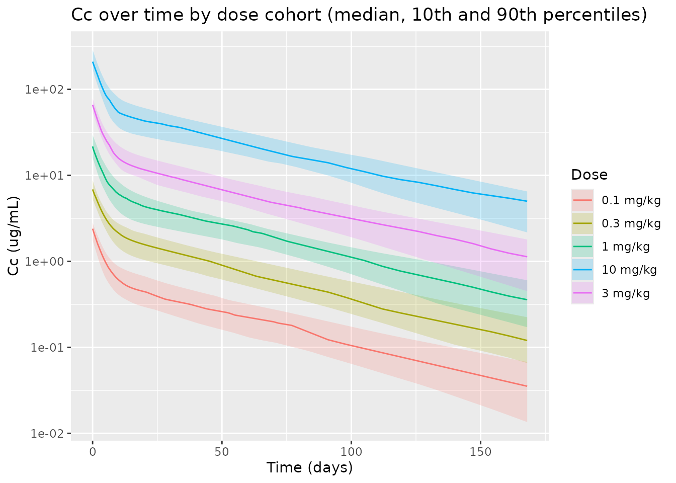
Concentration-time curves by dose
A complementary view shows median concentrations per dose group on a log y-axis. The proportional spacing of the curves and the parallel terminal slopes are consistent with linear two-compartment disposition as described in Nicholas 2009 Results (“The PK profile of PF-04360365 appeared linear”).
by_dose <- sim |>
  dplyr::filter(!is.na(Cc)) |>
  dplyr::mutate(time_day = time / 24,
                Cc       = ifelse(Cc > 0, Cc, NA_real_)) |>
  dplyr::group_by(treatment, dose_mgkg, time_day) |>
  dplyr::summarise(
    Q05 = stats::quantile(Cc, 0.10, na.rm = TRUE),
    Q50 = stats::quantile(Cc, 0.50, na.rm = TRUE),
    Q95 = stats::quantile(Cc, 0.90, na.rm = TRUE),
    .groups = "drop"
  )

ggplot(by_dose, aes(time_day, Q50, colour = treatment, fill = treatment)) +
  geom_ribbon(aes(ymin = Q05, ymax = Q95), alpha = 0.20, colour = NA) +
  geom_line() +
  scale_y_log10() +
  labs(
    x = "Time (days)",
    y = "Cc (ug/mL)",
    colour = "Dose",
    fill = "Dose",
    title = "Cc over time by dose cohort (median, 10th and 90th percentiles)"
  )
PKNCA validation
Nicholas 2009 does not tabulate NCA parameter values, so the PKNCA results below stand on their own as an internal validation of the simulation output: the proportionality of Cmax and AUC to dose confirms the linearity reported in the paper, and the terminal half-life is consistent with the disposition parameters in Table 1.
sim_nca <- sim |>
  dplyr::filter(!is.na(Cc)) |>
  dplyr::select(id, time, Cc, treatment)

# Guarantee a time = 0 row per (id, treatment); for an IV bolus delivered at
# time 0 the simulation already reports Cc at t = 0 (= dose / vc) but defend
# explicitly so the PKNCA AUC anchor is never lost.
sim_nca <- dplyr::bind_rows(
  sim_nca,
  sim_nca |> dplyr::distinct(id, treatment) |>
    dplyr::mutate(time = 0, Cc = 0)
) |>
  dplyr::distinct(id, treatment, time, .keep_all = TRUE) |>
  dplyr::arrange(id, treatment, time)

dose_df <- events |>
  dplyr::filter(evid == 1) |>
  dplyr::select(id, time, amt, treatment)

conc_obj <- PKNCA::PKNCAconc(
  sim_nca, Cc ~ time | treatment + id,
  concu = "ug/mL", timeu = "h"
)
dose_obj <- PKNCA::PKNCAdose(
  dose_df, amt ~ time | treatment + id,
  doseu = "mg"
)

intervals <- data.frame(
  start       = 0,
  end         = Inf,
  cmax        = TRUE,
  tmax        = TRUE,
  aucinf.obs  = TRUE,
  half.life   = TRUE,
  clast.obs   = TRUE,
  lambda.z    = TRUE
)

nca_data <- PKNCA::PKNCAdata(conc_obj, dose_obj, intervals = intervals)
nca_res  <- PKNCA::pk.nca(nca_data)

nca_summary <- as.data.frame(nca_res$result) |>
  dplyr::group_by(treatment, PPTESTCD) |>
  dplyr::summarise(
    median = stats::median(PPORRES, na.rm = TRUE),
    q05    = stats::quantile(PPORRES, 0.05, na.rm = TRUE),
    q95    = stats::quantile(PPORRES, 0.95, na.rm = TRUE),
    .groups = "drop"
  ) |>
  dplyr::filter(PPTESTCD %in% c("cmax", "tmax", "aucinf.obs", "half.life")) |>
  dplyr::mutate(parameter = nlmixr2lib::ncaParamLabel(PPTESTCD)) |>
  dplyr::select(treatment, parameter, median, q05, q95)

knitr::kable(
  nca_summary,
  digits  = 3,
  caption = "Simulated NCA per dose cohort (median, 5th and 95th percentiles)."
)| treatment | parameter | median | q05 | q95 |
|---|---|---|---|---|
| 0.1 mg/kg | AUC0-∞ (obs) | 1050.902 | 613.673 | 1446.248 |
| 0.1 mg/kg | Cmax | 2.396 | 1.579 | 2.971 |
| 0.1 mg/kg | t½ | 1035.202 | 625.434 | 1403.955 |
| 0.1 mg/kg | Tmax | 0.000 | 0.000 | 0.000 |
| 0.3 mg/kg | AUC0-∞ (obs) | 3450.033 | 2261.395 | 5175.814 |
| 0.3 mg/kg | Cmax | 6.863 | 5.184 | 9.001 |
| 0.3 mg/kg | t½ | 979.353 | 745.844 | 1228.773 |
| 0.3 mg/kg | Tmax | 0.000 | 0.000 | 0.000 |
| 1 mg/kg | AUC0-∞ (obs) | 10476.486 | 7027.789 | 12722.366 |
| 1 mg/kg | Cmax | 21.661 | 15.604 | 30.390 |
| 1 mg/kg | t½ | 996.327 | 732.396 | 1365.527 |
| 1 mg/kg | Tmax | 0.000 | 0.000 | 0.000 |
| 10 mg/kg | AUC0-∞ (obs) | 102000.707 | 78913.094 | 140779.845 |
| 10 mg/kg | Cmax | 209.720 | 163.761 | 297.831 |
| 10 mg/kg | t½ | 1089.342 | 753.141 | 1571.804 |
| 10 mg/kg | Tmax | 0.000 | 0.000 | 0.000 |
| 3 mg/kg | AUC0-∞ (obs) | 26209.590 | 20216.116 | 36549.136 |
| 3 mg/kg | Cmax | 65.986 | 52.691 | 81.093 |
| 3 mg/kg | t½ | 975.609 | 748.563 | 1387.755 |
| 3 mg/kg | Tmax | 0.000 | 0.000 | 0.000 |
A linearity check: Cmax and AUC0-inf should scale linearly with dose, within Monte Carlo noise.
linearity <- as.data.frame(nca_res$result) |>
  dplyr::filter(PPTESTCD %in% c("cmax", "aucinf.obs")) |>
  dplyr::left_join(
    subjects |> dplyr::select(id, dose_mgkg),
    by = "id"
  ) |>
  dplyr::group_by(dose_mgkg, PPTESTCD) |>
  dplyr::summarise(median = stats::median(PPORRES, na.rm = TRUE),
                   .groups = "drop") |>
  tidyr::pivot_wider(names_from = PPTESTCD, values_from = median) |>
  dplyr::mutate(
    cmax_per_mgkg       = cmax / dose_mgkg,
    aucinf_obs_per_mgkg = aucinf.obs / dose_mgkg
  )

knitr::kable(
  linearity,
  digits  = c(2, 3, 1, 4, 2),
  caption = "Dose-normalised median Cmax and AUC0-inf by cohort. Approximately constant values indicate linear disposition (Nicholas 2009 Results)."
)| dose_mgkg | aucinf.obs | cmax | cmax_per_mgkg | aucinf_obs_per_mgkg |
|---|---|---|---|---|
| 0.1 | 1050.902 | 2.4 | 23.9586 | 10509.02 |
| 0.3 | 3450.033 | 6.9 | 22.8759 | 11500.11 |
| 1.0 | 10476.486 | 21.7 | 21.6610 | 10476.49 |
| 3.0 | 26209.590 | 66.0 | 21.9954 | 8736.53 |
| 10.0 | 102000.707 | 209.7 | 20.9720 | 10200.07 |
Assumptions and deviations
- Body-weight distribution: the poster does not tabulate weights for the 26 subjects. The virtual cohort uses a truncated normal distribution centred at 70 kg (mean 70, SD 12, clamped to 50-100 kg) to span typical adult mild-to-moderate AD weights. The allometric reference weight 70 kg is taken from Nicholas 2009 Methods.
- Dose levels: the poster reports a single intravenous dose range of 0.1-10 mg/kg without specifying which dose levels were used. The virtual cohort uses 0.1, 0.3, 1, 3, and 10 mg/kg as representative single doses spanning the reported range.
- Sex, race / ethnicity, and region distributions are not tabulated in the poster and are not used as covariates in the model.
- Concentration units: the poster reports concentrations in ng/mL on the ELISA scale (analytical range 156-10,000 ng/mL). The model encodes concentrations as Cc = central / vc in mg/L = ug/mL given dose in mg and volume in L. Plots and tables therefore display ug/mL; multiplying by 1000 converts to ng/mL on the poster scale.
- The poster does not tabulate numerical NCA parameter values; the PKNCA section presents simulated NCA without a published reference for comparison.
- The poster notes that Theta_7 (allometric exponent on Q) and Theta_8 (allometric exponent on V2) are imprecisely estimated (95% CIs crossing or near zero). These point estimates are encoded as reported; the imprecision is documented in the source-trace table.
- IV bolus dosing is used in the simulation. The poster does not state whether the doses were given as bolus or short infusion; for a mAb the difference at typical sampling resolution is negligible, and the model is parameterised by CL/V1/Q/V2 without an explicit infusion compartment.