Polymyxin B (Li 2021)

Model and source

• Citation: Li Y, Deng Y, Zhu ZY, Liu YP, Xu P, Li X, Xie YL, Yao HC, Yang L, Zhang BK, Zhou YG. Population pharmacokinetics of polymyxin B and dosage optimization in renal transplant patients. Front Pharmacol. 2021;12:727170. doi:10.3389/fphar.2021.727170. PMCID PMC8424097.
• Description: One-compartment intravenous population PK model for polymyxin B in adult renal transplant recipients, most with renal dysfunction (Li 2021). Cockcroft-Gault creatinine clearance is a power covariate on clearance, normalized to the cohort median of 22.2 mL/min with exponent 0.14. Volume of distribution carries no covariate. Exponential IIV on CL and V; proportional residual error. Fit in Phoenix NLME (FOCE-ELS).
• Article: Front Pharmacol. 2021;12:727170

Population

Li 2021 is a prospective single-centre study (The Second Xiangya Hospital, Central South University, Changsha, China; ChiCTR1900022231) of 50 adult renal transplant recipients who received intravenous polymyxin B every 12 h as a 60-120 min infusion for at least 48 h. Table 1 gives a median age of 43.5 years (18-66), 18 women and 32 men, and an actual body weight of 57.8 +/- 12.4 kg. Renal function was poor: Cockcroft-Gault creatinine clearance had a median of 22.2 mL/min (range 4.29-90.7), 92% had CrCL <= 80 mL/min, 29 patients had CrCL < 30 mL/min, and 11 (22%) received continuous renal replacement therapy. The infection site was pulmonary in 90%. The commonest maintenance doses were 40 mg q12h (44%) and 50 mg q12h (40%); only two patients received a loading dose.

One to six samples per patient (151 in total, Table 2) were drawn 30 min before the sixth dose and at 0, 0.5, 1, 2, 4, 6 and 8 h after the end of that infusion. Polymyxin B1 and B2 were measured by HPLC-MS/MS (LLOQ 0.03 mg/L); observed concentrations ranged from 0.44 to 8.15 mg/L. The model was fit in Phoenix NLME 8.1 with FOCE-ELS.

The same information is available programmatically via the model’s population metadata (readModelDb("Li_2021_polymyxinB")()$population).

Source trace

The per-parameter origin is recorded as an in-file comment next to each ini() entry in inst/modeldb/specificDrugs/Li_2021_polymyxinB.R. The table below collects them in one place for review.

Equation / parameter	Value	Source location
lcl (CL)	1.18 L/h	Table 4, “CL (L/h)”; %CV 4.15, bootstrap 95% CI 1.08-1.27
lvc (V)	12.09 L	Table 4, “V (L)”; %CV 6.52, bootstrap 95% CI 10.71-13.67
e_crcl_cl	0.14	Table 4, “Theta CrCL”; %CV 29.35, bootstrap 95% CI 0.05-0.21
CRCL normalising constant	22.2 mL/min	Final-model equation (Results); equals the Table 1 median
etalcl	variance 0.0600	Table 4, “omega^2 CL” 0.06 (shrinkage 7.16%), %CV 24.49
etalvc	variance 0.0430	Table 4, “omega^2 V” 0.04 (shrinkage 40.70%), %CV 20.74
propSd	0.17	Table 4, “sigma”; bootstrap 95% CI 0.13-0.21; proportional model selected in Table 3
cl <- exp(lcl + etalcl) * (CRCL/22.2)^e_crcl_cl	n/a	Results: “CL (L/h) = 1.18(CrCL/22.2)^0.14exp(eta CL)”
vc <- exp(lvc + etalvc)	n/a	Results: “V (L) = 12.09*exp(eta V)”
d/dt(central) <- -kel * central	n/a	Results: “A one-compartment PK model with first-order elimination fit the best”
Cc ~ prop(propSd)	n/a	Results: “A proportional error model was used to evaluate the residual variability”
2-h infusion, regimens	n/a	Methods, “Monte Carlo Simulation”

The IIV variances

Table 4 prints the two IIV variances to only two decimals (0.04 and 0.06) and, in its %CV column, the CV percentages 20.74 and 24.49. That column is sqrt(omega^2) * 100: sqrt(0.06) is 0.2449 exactly, and the Discussion calls 24.49% “the interindividual variability of CL” of the final model (down from 28.11% before CrCL entered). The packaged variances are therefore the squares of the more precise CV column, 0.2074^2 = 0.0430 and 0.2449^2 = 0.0600, both of which round to the printed values. The Table 6 reconstruction below confirms the CL variance independently: the day-3 AUC percentiles depend only on clearance, and their P90/P10 spread is reproduced by omega = 0.2449.

Virtual cohort

The paper’s Monte Carlo simulations (Methods; Tables 5 and 6) evaluated five regimens, each a loading dose followed by a q12h maintenance dose given as a 2-h infusion, in three renal-function groups labelled CrCL <= 30, <= 50 and <= 80 mL/min. The between-group ratios of the published AUC medians match the power model evaluated exactly at 30, 50 and 80 mL/min (checked below), so each group is simulated at that single CrCL value. 100 virtual subjects are drawn per regimen-by-group arm.

# rxSetSeed() fixes rxode2's eta sampler within an rxode2 build, but not across
# builds or solver thread counts. Every assertion below is therefore written on
# a deterministic (zeroRe / closed-form) quantity or on a robust centre.
rxode2::rxSetSeed(20210825)

n_per_arm <- 100L
tau <- 12
t_inf <- 2
t_end <- 72

regimens <- tibble::tibble(
  regimen = c("50 + 30", "50 + 40", "75 + 50", "100 + 50", "150 + 75"),
  ld = c(50, 50, 75, 100, 150),
  md = c(30, 40, 50, 50, 75)
)
crcl_groups <- tibble::tibble(
  crcl_group = c("<= 30 mL/min", "<= 50 mL/min", "<= 80 mL/min"),
  CRCL = c(30, 50, 80)
)

arms <- tidyr::expand_grid(regimens, crcl_groups) |>
  dplyr::mutate(
    arm = paste0(regimen, " mg, ", crcl_group),
    arm_id = dplyr::row_number()
  )

subjects <- tidyr::expand_grid(arms, rep = seq_len(n_per_arm)) |>
  dplyr::mutate(id = dplyr::row_number())

# Loading dose at t = 0, maintenance doses every 12 h from t = 12, all written
# out explicitly (PKNCA does not expand addl).
dose_times <- seq(0, t_end - tau, by = tau)
dose_rows <- tidyr::expand_grid(subjects, time = dose_times) |>
  dplyr::mutate(amt = ifelse(time == 0, ld, md), evid = 1, cmt = "central",
                dur = t_inf)

obs_times <- seq(0, t_end, by = 0.25)
obs_rows <- tidyr::expand_grid(subjects, time = obs_times) |>
  dplyr::mutate(amt = NA_real_, evid = 0, cmt = "central", dur = NA_real_)

events <- dplyr::bind_rows(dose_rows, obs_rows) |>
  dplyr::arrange(id, time, dplyr::desc(evid)) |>
  dplyr::select(id, time, amt, evid, cmt, dur, CRCL, arm, regimen, crcl_group,
                ld, md) |>
  as.data.frame()

stopifnot(
  length(unique(events$id)) == nrow(arms) * n_per_arm,
  nrow(dose_rows) == nrow(subjects) * length(dose_times)
)

Simulation

mod <- readModelDb("Li_2021_polymyxinB")

sim_cohort <- rxode2::rxSolve(
  mod, events = events,
  keep = c("CRCL", "arm", "regimen", "crcl_group", "md")
) |>
  as.data.frame()
#> ℹ parameter labels from comments will be replaced by 'label()'

stopifnot(nrow(sim_cohort) == nrow(subjects) * length(obs_times))

A matching typical-value solve, one subject per arm, is used for the deterministic checks.

mod_typical <- rxode2::zeroRe(mod)
#> ℹ parameter labels from comments will be replaced by 'label()'

events_typical <- events |>
  dplyr::filter(id %in% subjects$id[subjects$rep == 1L])

sim_typical <- rxode2::rxSolve(
  mod_typical, events = events_typical,
  keep = c("CRCL", "arm", "regimen", "crcl_group", "md")
) |>
  as.data.frame()
#> ℹ omega/sigma items treated as zero: 'etalcl', 'etalvc'
#> Warning: multi-subject simulation without without 'omega'

# Concentration-time profiles for the five regimens in the CrCL <= 30 group.
sim_cohort |>
  dplyr::filter(crcl_group == "<= 30 mL/min") |>
  dplyr::group_by(regimen, time) |>
  dplyr::summarise(
    Q05 = stats::quantile(Cc, 0.05),
    Q50 = stats::median(Cc),
    Q95 = stats::quantile(Cc, 0.95),
    .groups = "drop"
  ) |>
  dplyr::mutate(regimen = factor(regimen, levels = regimens$regimen)) |>
  ggplot(aes(time, Q50)) +
  geom_ribbon(aes(ymin = Q05, ymax = Q95), alpha = 0.25) +
  geom_line() +
  facet_wrap(~regimen, labeller = labeller(regimen = function(x) paste(x, "mg"))) +
  scale_x_continuous(breaks = seq(0, 72, by = 12)) +
  labs(x = "Time (h)", y = "Polymyxin B concentration (mg/L)",
       caption = paste("Loading + q12h maintenance dose, 2-h infusions, CrCL 30 mL/min;",
                       "median and 5th-95th percentile of 100 virtual subjects per regimen."))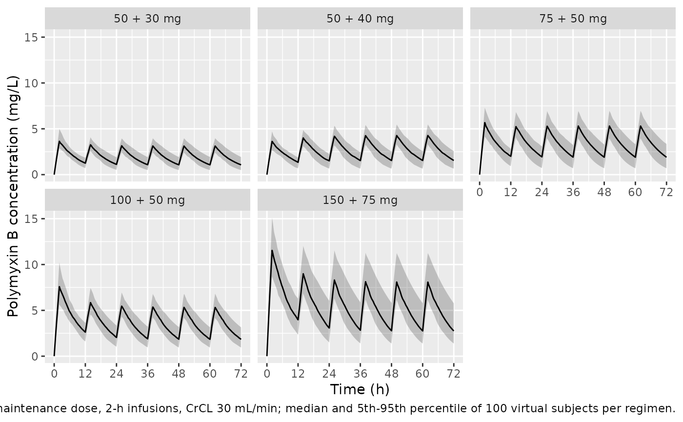

PKNCA validation

Table 6 reports AUC0-24h on day 1 (0-24 h) and day 3 (48-72 h). Both windows are computed with PKNCA, grouped by arm.

sim_nca <- sim_cohort |>
  dplyr::filter(!is.na(Cc)) |>
  dplyr::select(id, time, Cc, arm)

stopifnot(all(tapply(sim_nca$time, sim_nca$id, function(x) any(x == 0))))

conc_obj <- PKNCA::PKNCAconc(sim_nca, Cc ~ time | arm + id,
                             concu = "mg/L", timeu = "h")
dose_df <- events |>
  dplyr::filter(evid == 1) |>
  dplyr::select(id, time, amt, arm)
dose_obj <- PKNCA::PKNCAdose(dose_df, amt ~ time | arm + id, doseu = "mg")

intervals <- data.frame(
  start = c(0, 48),
  end = c(24, 72),
  auclast = TRUE,
  cmax = TRUE
)

nca_res <- PKNCA::pk.nca(PKNCA::PKNCAdata(conc_obj, dose_obj,
                                          intervals = intervals))

nca_long <- as.data.frame(nca_res) |>
  dplyr::mutate(day = ifelse(start == 0, "Day 1", "Day 3")) |>
  dplyr::left_join(dplyr::distinct(arms, arm, regimen, crcl_group, CRCL, md),
                   by = "arm")

auc_long <- nca_long |>
  dplyr::filter(PPTESTCD == "auclast")

stopifnot(nrow(auc_long) == 2L * nrow(subjects))

Solve against its own closed form

For a linear one-compartment model at steady state, AUC over a 24-h window is the 24-h maintenance dose divided by the individual clearance. Day 3 is close to, but not exactly at, steady state for subjects whose drawn CL and V give a long half-life, so this is checked on the centre and a robust quantile rather than on the worst subject.

cl_i <- sim_cohort |>
  dplyr::group_by(id) |>
  dplyr::summarise(cl = dplyr::first(cl), .groups = "drop")

auc_chk <- auc_long |>
  dplyr::filter(day == "Day 3") |>
  dplyr::inner_join(cl_i, by = "id") |>
  dplyr::mutate(
    auc_closed_form = 2 * md / cl,
    pct_diff = 100 * (PPORRES - auc_closed_form) / auc_closed_form
  )

knitr::kable(
  tibble::tibble(
    Statistic = c("Median % difference", "90th percentile |% difference|"),
    Value = c(stats::median(auc_chk$pct_diff),
              stats::quantile(abs(auc_chk$pct_diff), 0.9))
  ),
  digits = 3,
  caption = "PKNCA day-3 AUC(48-72) against 24-h maintenance dose / individual CL."
)

PKNCA day-3 AUC(48-72) against 24-h maintenance dose / individual CL.

Statistic	Value
Median % difference	0.023
90th percentile |% difference|	0.367

stopifnot(
  abs(stats::median(auc_chk$pct_diff)) < 1,
  stats::quantile(abs(auc_chk$pct_diff), 0.9) < 3
)

Comparison against published Table 6

# Li 2021 Table 6, transcribed: AUC0-24h (mg h/L) percentiles by regimen,
# renal-function group and day.
table6_pub <- tibble::tribble(
  ~regimen,   ~day,    ~crcl_group,     ~P10,   ~P50,   ~P90,
  "50 + 30",  "Day 1", "<= 30 mL/min",  39.73,  51.60,  65.64,
  "50 + 30",  "Day 1", "<= 50 mL/min",  37.74,  49.37,  63.15,
  "50 + 30",  "Day 1", "<= 80 mL/min",  35.90,  47.27,  60.74,
  "50 + 30",  "Day 3", "<= 30 mL/min",  34.37,  46.18,  63.67,
  "50 + 30",  "Day 3", "<= 50 mL/min",  32.11,  43.26,  59.85,
  "50 + 30",  "Day 3", "<= 80 mL/min",  30.18,  40.65,  56.43,
  "50 + 40",  "Day 1", "<= 30 mL/min",  43.29,  56.75,  71.78,
  "50 + 40",  "Day 1", "<= 50 mL/min",  41.03,  54.24,  68.76,
  "50 + 40",  "Day 1", "<= 80 mL/min",  39.11,  51.93,  66.02,
  "50 + 40",  "Day 3", "<= 30 mL/min",  45.57,  61.27,  83.15,
  "50 + 40",  "Day 3", "<= 50 mL/min",  42.60,  57.30,  77.92,
  "50 + 40",  "Day 3", "<= 80 mL/min",  40.07,  53.92,  73.42,
  "75 + 50",  "Day 1", "<= 30 mL/min",  61.56,  79.90, 101.10,
  "75 + 50",  "Day 1", "<= 50 mL/min",  56.30,  75.88,  96.75,
  "75 + 50",  "Day 1", "<= 80 mL/min",  55.62,  72.94,  92.92,
  "75 + 50",  "Day 3", "<= 30 mL/min",  56.97,  76.72, 104.44,
  "75 + 50",  "Day 3", "<= 50 mL/min",  53.26,  71.73,  97.78,
  "75 + 50",  "Day 3", "<= 80 mL/min",  50.07,  67.43,  91.99,
  "100 + 50", "Day 1", "<= 30 mL/min",  75.51,  97.73, 123.83,
  "100 + 50", "Day 1", "<= 50 mL/min",  71.71,  93.22, 118.47,
  "100 + 50", "Day 1", "<= 80 mL/min",  68.41,  89.08, 113.60,
  "100 + 50", "Day 3", "<= 30 mL/min",  57.02,  76.97, 105.29,
  "100 + 50", "Day 3", "<= 50 mL/min",  53.29,  71.91,  98.57,
  "100 + 50", "Day 3", "<= 80 mL/min",  50.08,  67.57,  92.60,
  "150 + 75", "Day 1", "<= 30 mL/min", 113.26, 146.59, 185.74,
  "150 + 75", "Day 1", "<= 50 mL/min", 104.15, 139.12, 177.55,
  "150 + 75", "Day 1", "<= 80 mL/min", 102.62, 133.61, 170.41,
  "150 + 75", "Day 3", "<= 30 mL/min",  85.65, 115.66, 158.32,
  "150 + 75", "Day 3", "<= 50 mL/min",  79.94, 107.87, 147.85,
  "150 + 75", "Day 3", "<= 80 mL/min",  71.57, 100.47, 138.51
) |>
  dplyr::mutate(arm = paste0(regimen, " mg, ", crcl_group))
stopifnot(nrow(table6_pub) == 30L)

# ncaComparisonTable() takes the per-subject median within each arm and day.
sim_for_cmp <- auc_long |>
  dplyr::select(arm, day, PPTESTCD, PPORRES)

ref_for_cmp <- table6_pub |>
  dplyr::transmute(arm, day, auclast = P50)

cmp <- nlmixr2lib::ncaComparisonTable(
  simulated = sim_for_cmp,
  reference = ref_for_cmp,
  by = c("arm", "day"),
  units = c(auclast = "mg*h/L"),
  tolerance_pct = 20
)

knitr::kable(
  cmp,
  caption = paste("Simulated median AUC0-24h against the P50 of Li 2021 Table 6,",
                  "by regimen (loading + maintenance, mg), CrCL group and day.",
                  "* differs from reference by >20%.")
)

Simulated median AUC0-24h against the P50 of Li 2021 Table 6, by regimen (loading + maintenance, mg), CrCL group and day. * differs from reference by >20%.

NCA parameter	arm	day	Reference	Simulated	% diff
AUClast (mg*h/L)	50 + 30 mg, <= 30 mL/min	Day 1	51.6	50.4	-2.3%
AUClast (mg*h/L)	50 + 30 mg, <= 30 mL/min	Day 3	46.2	46.1	-0.2%
AUClast (mg*h/L)	50 + 30 mg, <= 50 mL/min	Day 1	49.4	49.7	+0.7%
AUClast (mg*h/L)	50 + 30 mg, <= 50 mL/min	Day 3	43.3	43.9	+1.6%
AUClast (mg*h/L)	50 + 30 mg, <= 80 mL/min	Day 1	47.3	48.3	+2.1%
AUClast (mg*h/L)	50 + 30 mg, <= 80 mL/min	Day 3	40.6	43.7	+7.6%
AUClast (mg*h/L)	50 + 40 mg, <= 30 mL/min	Day 1	56.8	58.6	+3.2%
AUClast (mg*h/L)	50 + 40 mg, <= 30 mL/min	Day 3	61.3	65.3	+6.6%
AUClast (mg*h/L)	50 + 40 mg, <= 50 mL/min	Day 1	54.2	56	+3.2%
AUClast (mg*h/L)	50 + 40 mg, <= 50 mL/min	Day 3	57.3	62.3	+8.8%
AUClast (mg*h/L)	50 + 40 mg, <= 80 mL/min	Day 1	51.9	51	-1.8%
AUClast (mg*h/L)	50 + 40 mg, <= 80 mL/min	Day 3	53.9	54.2	+0.4%
AUClast (mg*h/L)	75 + 50 mg, <= 30 mL/min	Day 1	79.9	80.8	+1.1%
AUClast (mg*h/L)	75 + 50 mg, <= 30 mL/min	Day 3	76.7	80.8	+5.3%
AUClast (mg*h/L)	75 + 50 mg, <= 50 mL/min	Day 1	75.9	77.9	+2.6%
AUClast (mg*h/L)	75 + 50 mg, <= 50 mL/min	Day 3	71.7	75.2	+4.8%
AUClast (mg*h/L)	75 + 50 mg, <= 80 mL/min	Day 1	72.9	71.1	-2.5%
AUClast (mg*h/L)	75 + 50 mg, <= 80 mL/min	Day 3	67.4	66.1	-2.0%
AUClast (mg*h/L)	100 + 50 mg, <= 30 mL/min	Day 1	97.7	99.4	+1.7%
AUClast (mg*h/L)	100 + 50 mg, <= 30 mL/min	Day 3	77	80.8	+5.0%
AUClast (mg*h/L)	100 + 50 mg, <= 50 mL/min	Day 1	93.2	93.9	+0.7%
AUClast (mg*h/L)	100 + 50 mg, <= 50 mL/min	Day 3	71.9	73	+1.5%
AUClast (mg*h/L)	100 + 50 mg, <= 80 mL/min	Day 1	89.1	91.2	+2.4%
AUClast (mg*h/L)	100 + 50 mg, <= 80 mL/min	Day 3	67.6	72	+6.6%
AUClast (mg*h/L)	150 + 75 mg, <= 30 mL/min	Day 1	147	150	+2.4%
AUClast (mg*h/L)	150 + 75 mg, <= 30 mL/min	Day 3	116	123	+5.9%
AUClast (mg*h/L)	150 + 75 mg, <= 50 mL/min	Day 1	139	143	+2.6%
AUClast (mg*h/L)	150 + 75 mg, <= 50 mL/min	Day 3	108	115	+6.3%
AUClast (mg*h/L)	150 + 75 mg, <= 80 mL/min	Day 1	134	133	-0.1%
AUClast (mg*h/L)	150 + 75 mg, <= 80 mL/min	Day 3	100	103	+2.6%

The stochastic medians above scatter by a few percent either way, because each arm has only 100 subjects. The deterministic typical-value solve below removes that noise. It sits above the published P50 in every cell: by 2.3-3.6% on day 1 and by 4.5-6.1% on day 3, with about the same offset in every regimen and renal-function group. An offset that is the same size everywhere cannot come from the CrCL exponent or from the group values. It corresponds to a clearance about 5% higher in the paper’s simulation than the printed final-model equation gives. The paper does not report enough simulation detail to identify the source (the shift is larger than the difference between the two CrCL medians it quotes, 22.2 and 20.89 mL/min). The model is shipped as published.

typ_auc <- sim_typical |>
  dplyr::group_by(arm, regimen, crcl_group, CRCL, md) |>
  dplyr::summarise(
    cl_typ = dplyr::first(cl),
    auc_d1 = {
      x <- time <= 24
      sum(diff(time[x]) * (utils::head(Cc[x], -1) + utils::tail(Cc[x], -1)) / 2)
    },
    .groups = "drop"
  ) |>
  dplyr::mutate(auc_d3 = 2 * md / cl_typ)

typ_cmp <- typ_auc |>
  tidyr::pivot_longer(c(auc_d1, auc_d3), names_to = "day",
                      values_to = "typical") |>
  dplyr::mutate(day = ifelse(day == "auc_d1", "Day 1", "Day 3")) |>
  dplyr::inner_join(dplyr::select(table6_pub, arm, day, P50), by = c("arm", "day")) |>
  dplyr::mutate(pct_diff = 100 * (typical - P50) / P50)

typ_cmp |>
  dplyr::group_by(day) |>
  dplyr::summarise(
    `Median % difference` = stats::median(pct_diff),
    `Min % difference` = min(pct_diff),
    `Max % difference` = max(pct_diff),
    .groups = "drop"
  ) |>
  dplyr::rename("Window" = day) |>
  knitr::kable(digits = 2,
               caption = "Typical-value AUC0-24h against the Table 6 P50, over the 15 regimen-by-group cells per day.")

Typical-value AUC0-24h against the Table 6 P50, over the 15 regimen-by-group cells per day.

Window	Median % difference	Min % difference	Max % difference
Day 1	2.95	2.28	3.55
Day 3	5.37	4.54	6.08

# Between-group ratios: these depend only on the CrCL exponent and the group
# CrCL values, and are what identifies the groups as CrCL = 30 / 50 / 80.
ratio_cmp <- typ_cmp |>
  dplyr::filter(day == "Day 3") |>
  dplyr::group_by(regimen) |>
  dplyr::mutate(
    ratio_typ = typical / typical[CRCL == 30],
    ratio_pub = P50 / P50[CRCL == 30]
  ) |>
  dplyr::ungroup() |>
  dplyr::filter(CRCL != 30)

# Spread: the day-3 P90/P10 ratio depends only on the CL variance.
spread_pub <- table6_pub |>
  dplyr::filter(day == "Day 3") |>
  dplyr::mutate(ratio = P90 / P10)
spread_model <- exp(2 * stats::qnorm(0.9) * sqrt(0.0600))

# Stochastic cohort: per-arm median AUC against the Table 6 P50.
sim_med_diff <- auc_long |>
  dplyr::group_by(arm, day) |>
  dplyr::summarise(sim_p50 = stats::median(PPORRES), .groups = "drop") |>
  dplyr::inner_join(dplyr::select(table6_pub, arm, day, P50), by = c("arm", "day")) |>
  dplyr::mutate(pct_diff = 100 * (sim_p50 - P50) / P50)
stopifnot(nrow(sim_med_diff) == 30L)

stopifnot(
  # Deterministic: the typical value sits above every published P50, by
  # 2-4% on day 1 and 4-7% on day 3 (the ranges quoted in the text).
  all(typ_cmp$pct_diff[typ_cmp$day == "Day 1"] > 2),
  all(typ_cmp$pct_diff[typ_cmp$day == "Day 1"] < 4),
  all(typ_cmp$pct_diff[typ_cmp$day == "Day 3"] > 4),
  all(typ_cmp$pct_diff[typ_cmp$day == "Day 3"] < 7),
  # Between-group ratios reproduce to 1%.
  all(abs(ratio_cmp$ratio_typ / ratio_cmp$ratio_pub - 1) < 0.01),
  # Day-3 spread from omega^2 CL = 0.0600 within 5% of every published P90/P10.
  all(abs(spread_model / spread_pub$ratio - 1) < 0.05),
  # Stochastic cohort: robust centre only.
  abs(stats::median(sim_med_diff$pct_diff)) < 8,
  stats::quantile(abs(sim_med_diff$pct_diff), 0.9) < 12
)

sim_pct <- auc_long |>
  dplyr::group_by(regimen, crcl_group, day) |>
  dplyr::summarise(
    P10 = stats::quantile(PPORRES, 0.1),
    P50 = stats::median(PPORRES),
    P90 = stats::quantile(PPORRES, 0.9),
    .groups = "drop"
  ) |>
  dplyr::mutate(source = "Simulated")

dplyr::bind_rows(sim_pct,
                 dplyr::mutate(dplyr::select(table6_pub, -arm), source = "Li 2021 Table 6")) |>
  dplyr::mutate(regimen = factor(regimen, levels = regimens$regimen)) |>
  ggplot(aes(regimen, P50, colour = source)) +
  geom_pointrange(aes(ymin = P10, ymax = P90),
                  position = position_dodge(width = 0.5)) +
  geom_hline(yintercept = c(50, 100), linetype = "dashed") +
  facet_grid(day ~ crcl_group) +
  labs(x = "Loading + maintenance dose (mg)", y = "AUC0-24h (mg h/L)",
       colour = NULL,
       caption = "Replicates Table 6 of Li 2021: median and 10th-90th percentile; dashed lines mark the 50-100 mg h/L target.") +
  theme(axis.text.x = element_text(angle = 45, hjust = 1), legend.position = "bottom")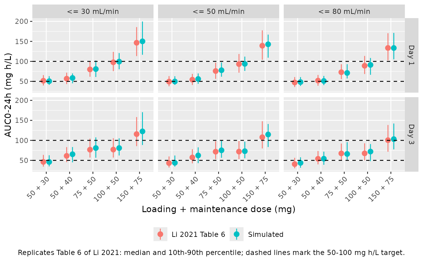

Table 5 – probability of target attainment on day 3

Table 5 reports, for CrCL 10 to 80 mL/min, the probability that fAUC0-24h/MIC >= 20 on day 3, with an unbound fraction of 0.42 (Methods). At day 3 the AUC is set by clearance alone, which is log-normal about the typical value, so each cell follows in closed form from the typical clearance (read off a zeroRe() solve) and omega.

pta_grid <- tidyr::expand_grid(regimens, CRCL = seq(10, 80, by = 10)) |>
  dplyr::mutate(id = dplyr::row_number())

pta_events <- pta_grid |>
  dplyr::transmute(id, time = 0, amt = NA_real_, evid = 0, cmt = "central",
                   dur = NA_real_, CRCL) |>
  as.data.frame()

pta_cl <- rxode2::rxSolve(mod_typical, events = pta_events) |>
  as.data.frame() |>
  dplyr::select(id, cl_typ = cl)
#> ℹ omega/sigma items treated as zero: 'etalcl', 'etalvc'
#> Warning: multi-subject simulation without without 'omega'

fu <- 0.42
omega_cl <- sqrt(0.0600)

pta_sim <- pta_grid |>
  dplyr::inner_join(pta_cl, by = "id") |>
  tidyr::expand_grid(MIC = c(0.5, 1, 2)) |>
  dplyr::mutate(
    auc_typ = 2 * md / cl_typ,
    pta = 1 - stats::pnorm(log(20 * MIC / fu / auc_typ) / omega_cl)
  )

# Li 2021 Table 5, transcribed. For each regimen, the eight CrCL rows
# (10, 20, ..., 80 mL/min) at MIC 0.5, 1 and 2 mg/L.
table5_pub <- tidyr::expand_grid(
  regimen = regimens$regimen,
  CRCL = seq(10, 80, by = 10),
  MIC = c(0.5, 1, 2)
) |>
  dplyr::mutate(published = c(
    1, .83, .02, 1, .72, .01, 1, .64, 0, 1, .57, 0, 1, .53, 0, 1, .48, 0, 1, .45, 0, 1, .43, 0,
    1, 1, .10, 1, 1, .04, 1, 1, .03, 1, 1, .02, 1, 1, .02, 1, 1, .01, 1, 1, .01, 1, 1, .01,
    1, 1, .38, 1, 1, .25, 1, 1, .18, 1, 1, .15, 1, 1, .12, 1, 1, .10, 1, 1, .09, 1, 1, .07,
    1, 1, .39, 1, 1, .26, 1, 1, .19, 1, 1, .15, 1, 1, .13, 1, 1, .11, 1, 1, .09, 1, 1, .08,
    1, 1, .92, 1, 1, .85, 1, 1, .79, 1, 1, .74, 1, 1, .70, 1, 1, .67, 1, 1, .63, 1, 1, .58
  ))
stopifnot(nrow(table5_pub) == 120L)

pta_cmp <- table5_pub |>
  dplyr::inner_join(dplyr::select(pta_sim, regimen, CRCL, MIC, pta),
                    by = c("regimen", "CRCL", "MIC")) |>
  dplyr::mutate(diff = pta - published)
stopifnot(nrow(pta_cmp) == 120L)

pta_cmp |>
  dplyr::filter(MIC > 0.5) |>
  dplyr::mutate(cell = sprintf("%.2f (%.2f)", pta, published)) |>
  dplyr::select(regimen, CRCL, MIC, cell) |>
  tidyr::pivot_wider(names_from = regimen, values_from = cell) |>
  dplyr::rename("CrCL (mL/min)" = CRCL, "MIC (mg/L)" = MIC) |>
  knitr::kable(caption = paste("Closed-form day-3 PTA for fAUC0-24h/MIC >= 20,",
                               "with the Li 2021 Table 5 value in parentheses.",
                               "Columns are loading + maintenance dose (mg).",
                               "At MIC 0.5 mg/L every published cell is 1 and",
                               "every closed-form cell is at least 0.99."))

Closed-form day-3 PTA for fAUC0-24h/MIC >= 20, with the Li 2021 Table 5 value in parentheses. Columns are loading + maintenance dose (mg). At MIC 0.5 mg/L every published cell is 1 and every closed-form cell is at least 0.99.

CrCL (mL/min)	MIC (mg/L)	50 + 30	50 + 40	75 + 50	100 + 50	150 + 75
10	1	0.77 (0.83)	0.97 (1.00)	1.00 (1.00)	1.00 (1.00)	1.00 (1.00)
10	2	0.02 (0.02)	0.18 (0.10)	0.49 (0.38)	0.49 (0.39)	0.95 (0.92)
20	1	0.63 (0.72)	0.93 (1.00)	0.99 (1.00)	0.99 (1.00)	1.00 (1.00)
20	2	0.01 (0.01)	0.09 (0.04)	0.34 (0.25)	0.34 (0.26)	0.89 (0.85)
30	1	0.54 (0.64)	0.90 (1.00)	0.99 (1.00)	0.99 (1.00)	1.00 (1.00)
30	2	0.00 (0.00)	0.06 (0.03)	0.26 (0.18)	0.26 (0.19)	0.84 (0.79)
40	1	0.47 (0.57)	0.87 (1.00)	0.98 (1.00)	0.98 (1.00)	1.00 (1.00)
40	2	0.00 (0.00)	0.04 (0.02)	0.21 (0.15)	0.21 (0.15)	0.80 (0.74)
50	1	0.42 (0.53)	0.84 (1.00)	0.97 (1.00)	0.97 (1.00)	1.00 (1.00)
50	2	0.00 (0.00)	0.03 (0.02)	0.17 (0.12)	0.17 (0.13)	0.76 (0.70)
60	1	0.38 (0.48)	0.81 (1.00)	0.96 (1.00)	0.96 (1.00)	1.00 (1.00)
60	2	0.00 (0.00)	0.03 (0.01)	0.15 (0.10)	0.15 (0.11)	0.73 (0.67)
70	1	0.35 (0.45)	0.78 (1.00)	0.96 (1.00)	0.96 (1.00)	1.00 (1.00)
70	2	0.00 (0.00)	0.02 (0.01)	0.13 (0.09)	0.13 (0.09)	0.70 (0.63)
80	1	0.32 (0.43)	0.76 (1.00)	0.95 (1.00)	0.95 (1.00)	1.00 (1.00)
80	2	0.00 (0.00)	0.02 (0.01)	0.11 (0.07)	0.11 (0.08)	0.67 (0.58)

Outside one column, the closed-form PTA tracks Table 5 to within about 0.1. The exception is the 50 + 40 mg regimen at MIC 1 mg/L, which Table 5 prints as 1 in every CrCL row. The model gives 0.76-0.97 there. Table 5 also disagrees with the paper’s own Table 6 here. Its day-3 P10 AUC for that regimen, 40.07 mg h/L in the CrCL <= 80 mL/min group, is below the 47.6 mg h/L that fAUC/MIC >= 20 needs at MIC 1 mg/L with fu = 0.42, so the PTA cannot be 1. The 50 + 40 mg MIC 1 cells are therefore reported but excluded from the gate.

pta_gate <- pta_cmp |>
  dplyr::filter(!(regimen == "50 + 40" & MIC == 1))
pta_lookup <- function(reg, crcl, mic) {
  pta_sim$pta[pta_sim$regimen == reg & pta_sim$CRCL == crcl & pta_sim$MIC == mic]
}

stopifnot(
  # Deterministic closed form: no random draw enters.
  stats::median(abs(pta_gate$diff)) < 0.02,
  stats::quantile(abs(pta_gate$diff), 0.9) < 0.11,
  max(abs(pta_gate$diff)) < 0.12,
  # Results: at MIC 2 mg/L only 150 + 75 mg in CrCL <= 10 mL/min reaches 90%.
  pta_lookup("150 + 75", 10, 2) >= 0.9,
  all(pta_sim$pta[pta_sim$MIC == 2 &
                    !(pta_sim$regimen == "150 + 75" & pta_sim$CRCL == 10)] < 0.9),
  # The MIC 0.5 mg/L claim made in the table caption.
  all(table5_pub$published[table5_pub$MIC == 0.5] == 1),
  all(pta_sim$pta[pta_sim$MIC == 0.5] >= 0.99),
  # The 50 + 40 mg MIC 1 mg/L range quoted in the text.
  all(round(pta_sim$pta[pta_sim$regimen == "50 + 40" & pta_sim$MIC == 1], 2) >= 0.76),
  all(round(pta_sim$pta[pta_sim$regimen == "50 + 40" & pta_sim$MIC == 1], 2) <= 0.97),
  # Maintenance doses >= 50 mg reach 90% at MIC <= 1 mg/L in every group.
  all(pta_sim$pta[pta_sim$md >= 50 & pta_sim$MIC <= 1] >= 0.9)
)

Assumptions and deviations

• IIV variances from the %CV column. Table 4 prints omega^2 to two decimals (0.04, 0.06). The packaged variances, 0.0430 and 0.0600, are the squares of the Table 4 %CV column (20.74% and 24.49%), which is sqrt(omega^2); see the source-trace section.
• Residual error on the SD scale. Phoenix NLME reports the residual epsilon as a standard deviation, so the Table 4 sigma of 0.17 is used directly as propSd.
• CrCL normalising constant. The final-model equation prints 22.2 mL/min, the Table 1 median. The Discussion quotes a different median, 20.89 mL/min (range 4.29-78.84). The printed equation is followed.
• Renal replacement therapy. Eleven patients (22%) received continuous renal replacement therapy. The paper neither screened CRRT as a covariate nor describes how CrCL was assigned during CRRT, so the model carries no RRT term.
• Simulation groups. Table 6 labels its renal-function groups “<= 30”, “<= 50” and “<= 80” mL/min. They are simulated here at exactly 30, 50 and 80 mL/min, which reproduces the published between-group ratios.
• Uniform offset from Table 6. The printed model gives typical-value AUCs 2.3-3.6% (day 1) and 4.5-6.1% (day 3) above the Table 6 medians in every cell. This is documented above and not adjusted.
• Table 5, 50 + 40 mg at MIC 1 mg/L. The printed PTA of 1 in every CrCL row is inconsistent with both the model and the paper’s own Table 6. It is reported and excluded from the gate. The Results text (“all regimens aside from a 50 mg loading dose with 40 mg every 12 h achieved the target concentration at MIC <= 1 mg/L”) also names the wrong regimen: Table 5 shows the 50 + 30 mg regimen falling short at MIC 1 mg/L.
• Observed AUC. The paper’s observed mean AUC0-24h (74.60 +/- 17.81 mg h/L, daily dose / individual CL) depends on the per-patient doses and CrCL values, which are not published, so it is not reproduced here.
• All parameter values come from the paper’s own text and tables. No value was taken from a figure, from correspondence, or from an upstream model.